
Daddy’s AP Calculus BC for Beth
posted: 01-Mar-2026 & updated: 16-Mar-2026
Share this on LinkedIn | Instagram | Twitter (X) | Facebook
Daily Practice Problems 🗓️
Beth’s daily warm-up sessions live on a separate page — short, casual, 15–20 minutes. Each session has problems + a collapsible answer key so you can self-check.
➡️ Beth’s Daily Calculus Practice
| Date | Topics |
|---|---|
| 16-Mar-2026 | Limits · Indeterminate forms · Series · Integration by parts · FTC both parts · Volumes |
| 15-Mar-2026 | Limits (higher-order · $0^0$ · $1^\infty$) · Series & radius of convergence · Integration by parts (solve for $I$!) · Volumes (mixed axes) |
| 11-Mar-2026 | Limits (two methods) · Series · Integration by parts · Volumes around $y$-axis (shell vs. washer) |
| 10-Mar-2026 | Limits (two methods) · Series · FTC + chain rule · Volumes of revolution (disc & shell) |
| 09-Mar-2026 | Limits at 0 and $\infty$ · Series convergence · FTC Part 1 |
Interactive Visualization Tools
- Interactive visualization - finite difference approximation
- Interactive visualization - Taylor approximation
- Interactive visualization - integral approximation
- Interactive visualization - arc length
- Interactive visualization — disc method
- Interactive 3D visualization — washer method
- Interactive 3D visualization — shell method
- Interactive 3D visualizations - volumes
- Interactive animation — watch the solution evolve in real time
- Power Functions
- Antiderivative of Power Functions
Important Topics, Patterns, and Rules
Differentiation / Derivatives
Definition
The derivative is a fundamental tool that quantifies the sensitivity to change of a function’s output with respect to its input. The derivative of a function of a single variable at a chosen input value, when it exists, is the slope of the tangent line to the graph of the function at that point. The tangent line is the best linear approximation of the function near that input value. The derivative is often described as the instantaneous rate of change, the ratio of the instantaneous change in the dependent variable to that of the independent variable. The process of finding a derivative is called differentiation.
A function of a real variable $\newcommand{\reals}{\mathbb{R}}\newcommand{\naturals}{\mathbb{N}}\newcommand{\series}{\sum_{n=1}^\infty a_n}\newcommand{\absseries}{\sum_{n=1}^\infty |a_n|}f(x)$ is differentiable at a point $a$ of its domain, if its domain contains an open interval containing $a$, and the limit in \eqref{eq:def-derivative} exists.
\begin{equation} \label{eq:def-derivative} \lim_{h\to 0} \frac{f(a+h)-f(a)}{h} \end{equation}
Examples
\[\begin{eqnarray} \label{eq:der-examples} \begin{array}{lcl} \dfrac{d}{dx} c &=& 0 \quad\mbox{for every } c \in \reals \\ \dfrac{d}{dx} x &=& 1 \\ \dfrac{d}{dx} x^2 &=& 2x \\ \dfrac{d}{dx} \left(\dfrac{1}{x}\right) &=& - \dfrac{1}{x^2} \\ \dfrac{d}{dx} \left(\dfrac{1}{x^2}\right) &=& - \dfrac{2}{x^3} \\ \dfrac{d}{dx} x^p &=& p x^{p-1} \quad\mbox{for every nonzero } p\in \reals \\ \dfrac{d}{dx} e^x &=& e^x \\ \dfrac{d}{dx} \ln x &=& \dfrac{1}{x} \\ \dfrac{d}{dx} \sin x &=& \cos x \\ \dfrac{d}{dx} \cos x &=& - \sin x \end{array} \end{eqnarray}\]Interactive visualization - finite difference approximations
The derivative is defined as a limit, but in practice we approximate it with finite differences. Watch how all three methods converge to the true tangent as $h \to 0$ — and notice how the centered difference is dramatically more accurate than the other two!
Chain rule
\begin{equation} \label{eq:chain-rule} \frac{d}{dx} f(g(x)) = f’(g(x)) g’(x) \end{equation}
We can recursively apply this to derive, e.g., the following rules.
\begin{equation} \label{eq:chain-rule-3} \frac{d}{dx} f(g(h(x))) = f’(g(h(x))) g’(h(x)) h’(x) \end{equation}
\begin{equation} \label{eq:chain-rule-4} \frac{d}{dx} f(g(h(p(x)))) = f’(g(h(p(x)))) g’(h(p(x))) h’(p(x)) p’(x) \end{equation}
\[\begin{eqnarray} \label{eq:chain-rule-5} \begin{array}{l} \dfrac{d}{dx} f(g(h(p(q(x))))) \\ = f'(g(h(p(q(x))))) g'(h(p(q(x)))) h'(p(q(x))) p'(q(x)) q'(x) \end{array} \end{eqnarray}\]And in general, for $n$ functions $f_1, f_2, \ldots, f_n$, the cursively applying the chain rule $n$ times yields
\[\begin{eqnarray} \label{eq:chain-rule-n} \begin{array}{rcl} \dfrac{d}{dx} f_1(f_2(\cdots f_n(x)\cdots)) &=& f_1'(f_2(\cdots f_n(x)\cdots)) f_2'(\cdots f_n(x)\cdots) \\ && \cdots f_{n-1}'(f_n(x)) f_n'(x) \end{array} \end{eqnarray}\]If we express this using the standard function composition notion $f \circ g$, i.e., $(f\circ g)(x)$ is defined to be $f(g(x))$,
\[\begin{eqnarray} \label{eq:chain-rule-n-fcn-comp} \begin{array}{rcl} \dfrac{d}{dx} (f_1\circ f_2\circ f_3\circ \cdots \circ f_n)(x) &=& f_1'( (f_2\circ f_3\circ \cdots \circ f_n)(x) ) \\ && f_2'( (f_3\circ \cdots \circ f_n)(x) ) \\ && \qquad \qquad \vdots \\ && f_{n-2}'((f_{n-1}\circ f_n)(x)) \\ && f_{n-1}'(f_n(x)) f_n'(x) \end{array} \end{eqnarray}\]Basic properties
For differentiable functions $f$ and $g$, and a constant $c$, the following rules hold.
Linearity
Differentiation is a linear operation!
\[(f + g)' = f' + g' \; \mbox{and} \; (cf)' = c f'\]So in one line
\begin{equation} \label{eq:der-linearity} (a f + b g)’ = a f’ + b g’ \end{equation}
This is arguably the single most useful structural fact about derivatives.
Product rule
The derivative of a product is not just $f’g’$!
\begin{equation} \label{eq:der-product-rule} (fg)’ = f’g + fg’ \end{equation}
A handy way to remember this – “derivative of first times second, plus first times derivative of second.”
Why the product rule matters for integration The product rule $(fg)’ = f’g + fg’$ can be rearranged as $f’g = (fg)’ - fg’$, and integrating both sides gives exactly the integration by parts formula — so the product rule is the parent of one of the most important integration techniques! We’ll see this connection in the integration section below.
Quotient rule
It follows directly from the chain rule and the product rule!
\begin{equation} \label{eq:der-quotient-rule} \left(\frac{f}{g}\right)’ = \frac{f’g - fg’}{g^2} \end{equation}
because the chain rule \eqref{eq:chain-rule} and the product rule \eqref{eq:der-product-rule} (together with basic derivative formulas in \eqref{eq:der-examples}) imply
\[\left(\frac{f}{g}\right)' = \left(f\cdot\frac{1}{g}\right)' = f' \left(\frac{1}{g}\right) + f \left(\frac{1}{g}\right)' = f' \cdot \frac{1}{g} - f \cdot \frac{g'}{g^2} = \frac{f'g - fg'}{g^2}\]A mnemonic – “low d-high minus high d-low, over low squared.”
Indeed, using the linearity of differentiation \eqref{eq:der-linearity} with the two rules, i.e., the chain rule \eqref{eq:chain-rule} and the product rule \eqref{eq:der-product-rule} (together with basic derivative formulas in \eqref{eq:der-examples}), we can derive every single formula related to differentiation in the whole universe! Actually, even in every multiverse! ★^^★1
Mean value theorem
The mean value theorem (or Lagrange’s mean value theorem) states, roughly, that for a given planar arc between two endpoints, there is at least one point at which the tangent to the arc is parallel to the secant through its endpoints. It is one of the most important results in real analysis.
Let $f:[a,b]\to\reals$ be a continuous function on the closed interval $[a,b]$, and differentiable on the open interval $(a,b)$, where $a< b$. Then there exists some $c$ in $(a,b)$ such that
\begin{equation} f’(c) = \frac{f(b)-f(a)}{b-a} \end{equation}
L’Hôpital’s rule
L’Hôpital’s rule states that for functions $f$ and $g$ which are defined on an open interval $I$ and differentiable on \(I\backslash\{c\}\) for a (possibly infinite) accumulation point $c$ of $I$, if
\[\lim_{x\to c} f(x) = \lim_{x\to c} g(x) = 0 \mbox{ or } \pm \infty\]and $\lim_{x\to c} \dfrac{f’(x)}{g’(x)}$ exists, then
\begin{equation} \label{eq:lhospital-rule} \lim_{x\to c} \frac{f(x)}{g(x)} = \lim_{x\to c} \frac{f’(x)}{g’(x)} \end{equation}
Examples
\[\begin{eqnarray*} \lim_{x\to 0} \frac{2x^2-3x}{3x^2+3x} &=& \lim_{x\to 0} \frac{4x-3}{6x+3} = -1 \\ \lim_{x\to \infty} \frac{2x^2+3x}{2+x^2} &=& \lim_{x\to \infty} \frac{2x+3}{2x} = \lim_{x\to \infty} \frac{2}{2} = 1 \\ \lim_{x\to 0} \frac{\sin(x)}{x} &=& \lim_{x\to 0} \frac{\cos(x)}{1} = 1 \\ \lim_{x\to \infty} xe^{-x} &=& \lim_{x\to \infty} \frac{x}{e^x} = \lim_{x\to \infty} \frac{1}{e^x} = 0 \\ \lim_{x\to \infty} x^2 e^{-x} &=& \lim_{x\to \infty} \frac{x^2}{e^x} = \lim_{x\to \infty} \frac{2x}{e^x} = \lim_{x\to \infty} \frac{2}{e^x} = 0 \\ \lim_{x\to \infty} \frac{\ln(x)}{x} &=& \lim_{x\to \infty} \frac{1/x}{1} = 0 \\ \lim_{x\to 0^+} x\ln x &=& \lim_{x\to 0^+} \frac{\ln(x)}{1/x} = \lim_{x\to 0^+} \frac{1/x}{-1/x^2} \\ &=& \lim_{x\to 0^+} (-x) = 0 \\ \lim_{x\to \infty} \frac{\ln(a+b\, e^{cx})}{x} &=& \lim_{x\to \infty} \frac{bc\, e^{cx}/(a+b\, e^{cx})}{1} \\ &=& c \quad \mbox{for } a,b,c>0 \\ \lim_{x\to 0} \frac{e^x-1}{x} &=& \lim_{x\to 0} \frac{e^x}{1} = 1 \\ \lim_{x\to 0} \frac{e^x-1}{x^2+x} &=& \lim_{x\to 0} \frac{e^x}{2x+1} = 1 \\ \lim_{x\to 0} \frac{2\sin x - \sin(2x)}{x-\sin x} &=& \lim_{x\to 0} \frac{2\cos x - 2\cos(2x)}{1-\cos x} \\ &=& \lim_{x\to 0} \frac{-2\sin x + 4\sin(2x)}{\sin x} \\ &=& \lim_{x\to 0} \frac{-2\cos x + 8\cos(2x)}{\cos x} = 6 \\ \lim_{h\to 0} \frac{f(x+h)+f(x-h)-2f(x)}{h^2} &=& \lim_{h\to 0} \frac{f(x+h)+f(x-h)-2f(x)}{h^2} \\ &=& \lim_{h\to 0} \frac{f'(x+h)-f'(x-h)}{2h} \\ &=& \lim_{h\to 0} \frac{f^{\prime\prime}(x+h)+f^{\prime\prime}(x-h)}{2} = f^{\prime\prime}(x) \end{eqnarray*}\]Caveat
\[\begin{eqnarray*} \lim_{x\to 0} \frac{x}{5} &\neq& \lim_{x\to 0} \frac{1}{0} \end{eqnarray*}\]Taylor series
The Taylor series or Taylor expansion of a function is an infinite sum of terms that are expressed in terms of the function’s derivatives at a single point. For most common functions, the function and the sum of its Taylor series are equal near this point. Taylor series are named after Brook Taylor, who introduced them in 1715. A Taylor series is also called a Maclaurin series when 0 is the point where the derivatives are considered, after Colin Maclaurin, who made extensive use of this special case of Taylor series in the 18th century.
The Taylor series of a real or complex-valued function $f(x)$, that is infinitely differentiable at a real or complex number $a$, is the power series
\begin{equation} \label{eq:taylor-series} \sum_{n=0}^\infty \frac{f^{(n)}(a)}{n!} (x-a)^n = f(a) + \frac{f’(a)}{1!}(x-a) + \frac{f^{\prime\prime}(a)}{2!}(x-a)^2 + \cdots \end{equation}
where $n!$ denotes the factorial of $n$, the function $f^{(n)}(a)$ denotes the $n$-th derivative of $f$ evaluated at the point $a$, the derivative of order zero of $f$ is defined to be $f$ itself, and $(x − a)^0$ and $0!$ are both defined to be $1$.
With $a = 0$, the Maclaurin series takes the form
\begin{equation} \label{eq:maclaurin-series} \sum_{n=0}^\infty \frac{f^{(n)}(0)}{n!} x^n = f(0) + \frac{f’(0)}{1!}x + \frac{f^{\prime\prime}(0)}{2!}x^2 + \cdots \end{equation}
Interactive visualization - Taylor approximation
Watch how each successive Taylor term sculpts the approximation closer and closer to the true curve. Drag the order slider to add terms one by one, and drag the center slider to move the expansion point $a$. Try different functions — $e^x$ converges everywhere, while $\ln(1+x)$ only converges for $|x| \le 1$!
Examples
\begin{equation} e^x = \sum_{n=0}^\infty \frac{x^n}{n!} = 1 + x + \frac{x^2}{2} + \frac{x^3}{3!} + \cdots \end{equation}
\begin{equation} \ln(1+x) = \sum_{n=0}^\infty (-1)^{n+1} \frac{x^n}{n} = x - \frac{x^2}{2} + \frac{x^3}{3} - \cdots \end{equation}
hence
\begin{equation} \ln(1-x) = - \sum_{n=0}^\infty (-1)^{n} \frac{x^n}{n} = - x - \frac{x^2}{2} - \frac{x^3}{3} - \cdots \end{equation}
\begin{equation} \frac{1}{1-x} = \sum_{n=0}^\infty x^n = 1 + x + x^2 + \cdots \end{equation}
\begin{equation} \frac{1}{(1-x)^2} = \sum_{n=1}^\infty nx^{n-1} = 1 + 2x + 3x^2 + \cdots \end{equation}
\[\begin{eqnarray} \sin(x) &=& \sum_{n=0}^\infty \frac{(-1)^n}{(2n+1)!} x^{2n+1} = x - \frac{x^3}{3!} + \frac{x^5}{5!} - \cdots \\ \cos(x) &=& \sum_{n=0}^\infty \frac{(-1)^n}{(2n)!} x^{2n} = 1 - \frac{x^2}{2!} + \frac{x^4}{4!} - \cdots \end{eqnarray}\]More examples can be shown in Taylor series Wikipedia Page!
Derivatives of trigonometric functions
\[\begin{eqnarray} \label{eq:der-tri} \begin{array}{rcl} \dfrac{d}{dx} \sin(x) &=& \cos(x) \\ \dfrac{d}{dx} \cos(x) &=& - \sin(x) \\ \dfrac{d}{dx} \tan(x) &=& \sec^2(x) = \dfrac{1}{\cos^2(x)} \\ \dfrac{d}{dx} \dfrac{1}{\tan(x)} = \dfrac{d}{dx} \cot(x) &=& - \csc^2(x) = - \dfrac{1}{\sin^2(x)} \\ \dfrac{d}{dx} \dfrac{1}{\cos(x)} = \dfrac{d}{dx} \sec(x) &=& \sec(x) \tan(x) = \dfrac{\sin(x)}{\cos^2(x)} \\ \dfrac{d}{dx} \dfrac{1}{\sin(x)} = \dfrac{d}{dx} \csc(x) &=& - \csc(x) \cot(x) = - \dfrac{\cos(x)}{\sin^2(x)} \end{array} \end{eqnarray}\]Derivatives of inverse trigonometric functions
\[\begin{eqnarray} \label{eq:der-inverse-tri} \begin{array}{rcl} \dfrac{d}{dx} \sin^{-1}(x) &=& \dfrac{1}{\sqrt{1-x^2}} \\ \dfrac{d}{dx} \cos^{-1}(x) &=& - \dfrac{1}{\sqrt{1-x^2}} \\ \dfrac{d}{dx} \tan^{-1}(x) &=& \dfrac{1}{1+x^2} \end{array} \end{eqnarray}\]More formula can be found here!
Integration / Integral
Riemann integral
The Riemann integral, created by Bernhard Riemann, was the first rigorous definition of the integral of a function on an interval. It was presented to the faculty at the University of Göttingen in 1854, but not published in a journal until 1868.
For many functions and practical applications, the Riemann integral can be evaluated by the Fundamental theorem of calculus or approximated by numerical integration, or simulated using Monte Carlo integration.
The big idea - slicing areas into rectangles
Imagine you want to find the area under a curve $f(x)$ between $x = a$ and $x = b$. The key idea is simple
slice the interval $[a, b]$ into $n$ thin vertical strips, approximate each strip as a rectangle, and add up all the rectangle areas!
As you use more and more slices (i.e., as $n \to \infty$), the approximation gets better and better — and in the limit, it becomes exact. That limit is precisely the definite integral!
\[\int_a^b f(x)\, dx = \lim_{n \to \infty} \sum_{i=1}^{n} f(x_i) \cdot \Delta x\]where $\Delta x = \dfrac{b-a}{n}$ is the width of each slice, and $x_i$ is any chosen point inside the $i$-th slice. The sum $\displaystyle\sum_{i=1}^{n} f(x_i) \cdot \Delta x$ is called a Riemann sum.
Four practical approximation methods (AP exam favorites!)
Depending on where you pick $x_i$ inside each slice, you get different approximation methods. The AP Calculus BC exam tests all four of these.
| Method | Where $x_i$ is chosen | Character |
|---|---|---|
| Left Riemann sum | Left endpoint of each slice | Underestimates if $f$ is increasing; overestimates if decreasing |
| Right Riemann sum | Right endpoint of each slice | Overestimates if $f$ is increasing; underestimates if decreasing |
| Midpoint rule | Midpoint of each slice | Generally more accurate than left or right |
| Trapezoidal rule | Uses trapezoids instead of rectangles | Exact for linear $f$; see formula below |
The trapezoidal rule replaces each rectangle with a trapezoid whose two parallel sides are $f(x_{i-1})$ and $f(x_i)$. This gives:
\begin{equation} \label{eq:trapezoidal-rule} \frac{\Delta x}{2} \left( f(x_0) + 2f(x_1) + 2f(x_2) + \cdots + 2f(x_{n-1}) + f(x_n) \right) \end{equation}
Note that the first and last terms have coefficient $1$, while all interior terms have coefficient $2$. Refer to LibreTexts - Numerical Integration - Midpoint, Trapezoid, Simpson’s rule for more details.
Over- or underestimate? It depends on concavity!
A key AP exam question type asks - “Is this approximation an overestimate or underestimate?” The answer depends on the concavity of $f$ on the interval:
- If $f$ is concave up ($f’’ > 0$): the trapezoidal rule overestimates, and the midpoint rule underestimates.
- If $f$ is concave down ($f’’ < 0$): the trapezoidal rule underestimates, and the midpoint rule overestimates.
For left/right Riemann sums, the over/underestimate depends on whether $f$ is increasing or decreasing (as shown in the table above).
Interactive visualization - integral approximation
Try it yourself, Beth! Drag the slider to increase $n$ and watch how the rectangles converge to the exact area. Toggle between methods to see Left, Right, Midpoint, and Trapezoidal approximations.
Basic properties
Linearity
Just like differentiation, integration is a linear operation:
\[\int \bigl(f(x) + g(x)\bigr)\, dx = \int f(x)\, dx + \int g(x)\, dx\] \[\int c\, f(x)\, dx = c \int f(x)\, dx\]So in one line
\begin{equation} \label{eq:int-linearity} \int \bigl(a f + b g\bigr)\, dx = a \int f\, dx + b \int g\, dx \end{equation}
This lets you split up and scale integrals freely — use it constantly!
Some useful properties to know
For definite integrals, a few more properties are worth knowing!
\begin{equation} \int_a^b f(x)\,dx = -\int_b^a f(x)\,dx \end{equation}
\begin{equation} \int_a^a f(x)\,dx = 0 \end{equation}
\begin{equation} \int_a^b f(x)\,dx = \int_a^c f(x)\,dx + \int_c^b f(x)\,dx \end{equation}
Integration by parts
Integration by parts is the integration counterpart of the product rule. Recall the product rule – $(fg)’ = f’g + fg’$. Integrating both sides and rearranging gives
\begin{equation} \label{eq:int-by-parts} \int f’(x)\, g(x)\, dx = f(x)g(x) - \int f(x)\, g’(x)\, dx \end{equation}
In the shorthand $u = g(x)$, $dv = f’(x)\,dx$ (so $v = f(x)$, $du = g’(x)\,dx$), this is the form you’ll see most often:
\begin{equation} \label{eq:int-by-parts-uv} \int u\, dv = uv - \int v\, du \end{equation}
The art of integration by parts is choosing $u$ and $dv$ smartly.
For definite integrals, we have
\begin{equation} \label{eq:int-by-parts-definite} \int_a^b f’(x)\, g(x)\, dx = \Bigl[f(x)g(x)\Bigr]_a^b - \int_a^b f(x)\, g’(x)\, dx \end{equation}
Examples
-
Find an indefinite integral $\displaystyle\int x e^x\,dx$
Solution 1 Choose $f(x) = e^x$ and $g(x) = x$. Then $f'(x) = e^x$ and $g'(x) = 1$, hence \eqref{eq:int-by-parts} gives \begin{equation} \label{eq:int-by-parts-exam-01} \int x e^x\, dx = x e^x - \int e^x\, dx = x e^x - e^x + C = (x-1)e^x + C \end{equation}
Solution 2 Choose $u = x$ and $v = e^x$. Then $du = dx$ and $dv = e^x dx$, thus \eqref{eq:int-by-parts-uv} gives $$ \int x e^x\, dx = x e^x - \int e^x\, dx = x e^x - e^x + C = (x-1)e^x + C $$
-
Find an indefinite integral $\displaystyle\int \ln x\,dx$
Solution 1 Choose $f(x) = x$ and $g(x) = \ln x$. Then $f'(x) = 1$ and $g'(x) = 1/x$, hence \eqref{eq:int-by-parts} gives $$ \int \ln x \, dx = x \ln x - \int 1\, dx = x \ln x - x + C $$
Solution 2 Choose $u = \ln x$ and $v = x$. Then $du = (1/x)dx$ and $dv = dx$, thus \eqref{eq:int-by-parts-uv} gives $$ \int \ln x \, dx = x \ln x - \int 1\, dx = x \ln x - x + C $$
-
Find an indefinite integral $\displaystyle\int x \sin x\,dx$
Solution 1 Choose $f(x) = -\cos x$ and $g(x) = x$. Then $f'(x) = \sin x$ and $g'(x) = 1$, hence \eqref{eq:int-by-parts} gives $$ \int x \sin x \, dx = - x \cos x + \int \cos x\, dx = - x \cos x + \sin x + C $$
Solution 2 Choose $u = x$ and $v = -\cos x$. Then $du = dx$ and $dv = \sin x dx$, thus \eqref{eq:int-by-parts-uv} gives $$ \int x \sin x \, dx = - x \cos x + \int \cos x\, dx = - x \cos x + \sin x + C $$
-
Find an indefinite integral $\displaystyle\int x^2 e^x \,dx$
Solution Choose $f(x) = e^x$ and $g(x) = x^2$. Then $f'(x) = e^x$ and $g'(x) = 2x$, hence \eqref{eq:int-by-parts} gives $$ \begin{eqnarray*} \int x^2 e^x \, dx &=& x^2 e^x - 2 \int x e^x \, dx = x^2 e^x - 2 (x-1) e^x + C \\ &=& (x^2 -2x+2)e^x + C \end{eqnarray*} $$ where \eqref{eq:int-by-parts-exam-01} is used
-
Find an indefinite integral $\displaystyle\int e^x \sin x \,dx$
Solution We let $\displaystyle I = \int e^x \sin x \,dx$. Now choose $f(x) = e^x$ and $g(x) = \sin x$. Then $f'(x) = e^x$ and $g'(x) = \cos x$, hence \eqref{eq:int-by-parts} gives \begin{equation} \label{eq:01} I = \int e^x \sin x \, dx = e^x \sin x - \int e^x \cos x \, dx \end{equation} Now to find $\displaystyle\int e^x \cos x \,dx$, we let $f(x) = e^x$ and $g(x) = \cos x$. Then $f'(x) = e^x$ and $g'(x) = - \sin x$, hence \begin{equation} \label{eq:02} \int e^x \cos x \, dx = e^x \cos x + \int e^x \sin x \, dx = e^x \cos x + I \end{equation} Now if we combine \eqref{eq:01} and \eqref{eq:02}, we have $$ I = e^x \sin x - e^x \cos x - I $$ thus, $$ \int e^x \sin x \, dx = I = \frac{1}{2} e^x (\sin x - \cos x) + C $$
- Find an indefinite integral $\displaystyle\int e^x \cos x \,dx$
- Find an indefinite integral $\displaystyle\int x \ln x \,dx$
Integration by Substitution
\begin{equation} \label{eq:int-by-sub} \int g’(x) f’(g(x)) dx = f(g(x)) + C \end{equation}
- Method 1 - using directly the chain rule, e.g., we just note that
\begin{equation} \label{eq:prob-int-by-sub-01} \int x e^{-x^2} dx = - \frac{1}{2} e^{-x^2} + C \end{equation}
- Method 2 - using u-substitution (also known as integration by substitution or substitution rule), i.e., by letting
then
\[du = g'(x) dx\]thus
\[\int g'(x) f'(g(x)) dx = \int f'(u) du = f(u) + C = f(g(x)) + C\]For example, to solve \eqref{eq:prob-int-by-sub-01}, we let $u=-x^2$, then we have $du = -2xdx$, hence
\[\int x e^{-x^2} dx = -\frac{1}{2} \int e^{u} du = -\frac{1}{2} e^{u} + C = -\frac{1}{2} e^{-x^2} + C\]which (of course) coincides with \eqref{eq:prob-int-by-sub-01}!
Integrals of inverse trigonometric functions
\[\begin{eqnarray} \label{eq:int-arcsin} \int \sin^{-1}(x) dx &=& x \sin^{-1}(x) + \sqrt{1-x^2} + C \\ \label{eq:int-arccos} \int \cos^{-1}(x) dx &=& x \cos^{-1}(x) - \sqrt{1-x^2} + C \\ \label{eq:int-arctan} \int \tan^{-1}(x) dx &=& x \tan^{-1}(x) - \frac{1}{2} \ln(x^2+1) + C \\ \label{eq:int-arcsin-a} \int \sin^{-1}(ax) dx &=& x \sin^{-1}(ax) + \frac{\sqrt{1-a^2x^2}}{a} + C \\ \nonumber \int \sin^{-1}(ax)^2 dx &=& -2x + x \sin^{-1}(ax)^2 \\ \label{eq:int-arcsin-squared} && \quad + \frac{2\sqrt{1-a^2x^2}\sin^{-1}(ax)}{a} + C \\ \label{eq:int-arccos-a} \int \cos^{-1}(ax) dx &=& x \cos^{-1}(ax) - \frac{\sqrt{1-a^2x^2}}{a} + C \\ \nonumber \int \cos^{-1}(ax)^2 dx &=& -2x + x \cos^{-1}(ax)^2 \\ \label{eq:int-arccos-squared} && \quad - \frac{2\sqrt{1-a^2x^2}\cos^{-1}(ax)}{a} + C \\ \label{eq:int-arctan-a} \int \tan^{-1}(ax) dx &=& x \tan^{-1}(ax) - \frac{\ln(a^2x^2+1)}{2a} + C \end{eqnarray}\]You can easily verify these formulas, e.g., using formulas in \eqref{eq:der-inverse-tri}. More formula can be found here!
Fundamental theorem of calculus
The fundamental theorem of calculus (FTC) is a theorem that links the concept of differentiating a function (calculating its slopes, or rate of change at every point on its domain) with the concept of integrating a function (calculating the area under its graph, or the cumulative effect of small contributions). Roughly speaking, the two operations can be thought of as inverses of each other.
The first part of the theorem, the first FTC, states that for a continuous function $f$, an antiderivative or indefinite integral $F$ can be obtained as the integral of $f$ over an interval with a variable upper bound.
Let $f$ be a continuous real-valued function defined on a closed interval $[a, b]$. Let $F$ be the function defined, for all $x$ in $[a, b]$, by
\[F(x) = \int_a^x f(t) \, dt\]Then $F$ is uniformly continuous on $[a, b]$ and differentiable on the open interval $(a, b)$, and
\[F'(x) = f(x)\]for all $x$ in $(a,b)$ so $F$ is an antiderivative of $f$. We can combine these two equations to write
\begin{equation} \label{eq:fund-theorem-of-calculus-1} \frac{d}{dx} \int_a^x f(t) \, dt = f(x) \end{equation}
Conversely, the second part of FTC (sometimes referred to as Newton–Leibniz theorem), states that the integral of a function $f$ over a fixed interval is equal to the change of any antiderivative $F$ between the ends of the interval.
Let $f$ be a real-valued function on a closed interval $[a,b]$ and $F$ a continuous function on $[a,b]$ which is an antiderivative of $f$ in $(a,b)$, i.e.,
\[F'(x) = f(x)\]Then if $f$ is Riemann integrable on $[a,b]$ then
\begin{equation} \label{eq:fund-theorem-of-calculus-2} \int_a^b f(x) \, dx = F(b) - F(a) \end{equation}
Examples using \eqref{eq:fund-theorem-of-calculus-1}
-
$$ \frac{d}{dx} \int_2^x \sqrt{1+t^2} \, dt = \sqrt{1+x^2} $$
-
$$ \lim_{h\to 0} \frac{\int_1^{1+h} \sqrt{x^5+8} \, dx}{h} = \sqrt{1^5+8} = 3 $$
-
$$ \frac{d}{dx} \int_a^{g(x)} f(t) \, dt = f(g(x)) g'(x) $$
-
$$ \frac{d}{dx} \int_{h(x)}^{g(x)} f(t) \, dt = f(g(x)) g'(x) - f(h(x)) h'(x) $$
-
$$ \frac{d}{dx} \int_2^{x^2} \sqrt{1+t^2} \, dt = 2x \sqrt{1+x^4} $$
Distance / Velocity / Acceleration / Length
One-dimensional case
In physics classes, we’ve learned movement of objects on a line, i.e., in one-dimensional line.
Suppose the location (or displacement) $d(t)\in\reals$, the velocity $v(t)\in\reals$, and the acceleration $a(t)\in\reals$ of an (rigid) object (or point mass). Then we have
\[\begin{eqnarray} \begin{array}{rcl} v(t) &=& d'(t) \\ &=& \dfrac{d}{dt} d(t) \end{array} \end{eqnarray}\] \[\begin{eqnarray} \begin{array}{rcl} a(t) &=& v'(t) = d^{\prime\prime}(t) \\ &=& \dfrac{d}{dt} v(t) = \dfrac{d^2}{dt^2} d(t) \end{array} \end{eqnarray}\]Therefore
\begin{equation} \label{eq:vel-int-dis-1} d(t) = \int_{t_0}^t v(\tau) d\tau + d(t_0) \end{equation}
and
\begin{equation} v(t) = \int_{t_0}^t a(\tau) d\tau + v(t_0) \end{equation}
Two-dimensional case
We can very naturally extend what we did in 1-dimensional line to a 2-dimensional plane with the concept of a vector and its representation using a Cartesian coordinate system.
Let $\vec{d}(t) = (x(t), y(t))\in\reals^2$ be the location of an object in a 2-dimensional space. Then the velocity $\vec{v}(t) = (v_x(t), v_y(t))\in\reals^2$ is
\begin{equation} (v_x(t), v_y(t)) = \dfrac{d}{dt} \vec{d}(t) = \left( \dfrac{d}{dt} x(t), \dfrac{d}{dt} y(t) \right) = (x’(t), y’(t)) \end{equation}
hence
\begin{equation} v_x(t) = x’(t),\quad v_y(t) = y’(t) \end{equation}
and the acceleration $\vec{a}(t) = (a_x(t), a_y(t)) \in\reals^2$ is
\begin{equation} (a_x(t), a_y(t)) = \frac{d}{dt} \vec{v}(t) = \left( \frac{d}{dt} v_x(t), \frac{d}{dt} v_y(t) \right) = (v_x’(t), v_y’(t)) \end{equation}
hence
\begin{equation} a_x(t) = v_x’(t) = x^{\prime\prime}(t),\quad a_y(t) = v_y’(t) = y^{\prime\prime}(t) \end{equation}
Therefore
\begin{equation} \vec{d}(t) = \int_{t_0}^t \vec{v}(\tau) d\tau + \vec{d}(t_0) \end{equation}
or equivalently
\begin{equation} (x(t),y(t)) = \int_{t_0}^t (x(\tau), y(\tau)) d\tau + (x(t_0), y(t_0)) \end{equation}
hence
\begin{equation} x(t) = \int_{t_0}^t v_x(\tau) d\tau + x(t_0),\; y(t) = \int_{t_0}^t v_y(\tau) d\tau + y(t_0) \end{equation}
Also
\begin{equation} \vec{v}(t) = \int_{t_0}^t \vec{a}(\tau) d\tau + \vec{v}(t_0) \end{equation}
or equivalently
\begin{equation} (v_x(t),v_y(t)) = \int_{t_0}^t (a_x(\tau), a_y(\tau)) d\tau + (v_x(t_0), v_y(t_0)) \end{equation}
hence
\begin{equation} v_x(t) = \int_{t_0}^t a_x(\tau) d\tau + v_x(t_0),\; v_y(t) = \int_{t_0}^t a_y(\tau) d\tau + v_y(t_0) \end{equation}
This can be also extended to the 3-dimensional case in a similar way.
Parameterized curve
The length of a curve parameterized by $(x(t),y(t))$ from $t=t_1$ to $t=t_2$ is
\begin{equation} \label{eq:vel-int-len} \mathrm{length} = \int_{t_1}^{t_2} \left|\vec{v}(t)\right| dt \end{equation}
because this can be thought of an object moving along a 1-dimensional curve, hence \eqref{eq:vel-int-dis-1} applies.
Interactive visualization - arc length
Watch how approximating the curve by $n$ straight chords converges to the true arc length $\int_{t_1}^{t_2} \lvert\vec{v}(t)\rvert\,dt$. The lower panel shows $\lvert\vec{v}(t)\rvert = \sqrt{x’(t)^2 + y’(t)^2}$ — its integral is exactly the arc length!
Area and Volume
Area
The area can be calculated by the integration of the length $l(x)$ of a cross section perpendicular to the $x$-axis, i.e.,
\begin{equation} A = \int_a^b l(x) dx \end{equation}
The area between two curves
\begin{equation} A = \int_a^b \left|f(x) - g(x)\right| dx \end{equation}
The area in polar coordinates
\begin{equation} A = \frac{1}{2} \int_\alpha^\beta r(\theta)^2 d\theta \end{equation}
The area between two polar curves
\begin{equation} A = \frac{1}{2} \int_\alpha^\beta (r_\mathrm{outer}(\theta)^2 - r_\mathrm{inner}(\theta)^2) d\theta \end{equation}
Volume
The volume can be calculated by the integration of the area $A(x)$ of a cross section perpendicular to the $x$-axis, i.e.,
\begin{equation} V = \int_a^b A(x) dx \end{equation}
Disc method for volume calculation
\begin{equation} \label{eq:vol-disc-method} V = \pi \int_a^b R(x)^2 dx \end{equation}
where $R(x)$ is the distance between the axis of revolution and the outside of the object
Interactive visualization — disc method
Washer method for volume calculation
\begin{equation} V = \pi \int_a^b \left( R(x)^2 - r(x)^2 \right)dx \end{equation}
where $R(x)$ is the radius of the outside of the object and $r(x)$ is the radius of the inside of the object
Interactive 3D visualization — washer method
Shell method for volume calculation
Shell integration (the shell method in integral calculus) is a method for calculating the volume of a solid of revolution, when integrating along an axis perpendicular to the axis of revolution. This is in contrast to disc integration which integrates along the axis parallel to the axis of revolution.
Consider a volume in three dimensions obtained by rotating a cross-section in the $xy$-plane around the $y$-axis. Suppose the cross-section is defined by the graph of the positive function $f(x)$ on the interval $[a, b]$. Then the formula for the volume will be
\begin{equation} \label{eq:vol-shell-method-rot-y} V = 2 \pi \int_a^b x f(x) dx \end{equation}
If the function is of the $y$ coordinate and the axis of rotation is the $x$-axis then the formula becomes
\begin{equation} \label{eq:vol-shell-method-rot-x} V = 2 \pi \int_a^b y f(y) dy \end{equation}
Interactive 3D visualization — shell method
Interactive 3D visualizations - volumes
Equilateral Triangle Cross-Sections
- The solid whose cross-sections perpendicular to the $x$-axis are equilateral triangles with side length $s = x^2$ for $x \in [0,2]$. $$ V = \frac{\sqrt{3}}{4} \int_{0}^{2} (x^2)^2 dx = \frac{\sqrt{3}}{4} \cdot \frac{1}{5} \Bigl.\Bigl(x^5\Bigr)\Bigr|_{x=0}^2 = \frac{8\sqrt{3}}{5} \simeq 2.7713 $$
-
The volume of the solid of revolution obtained
by rotating about the $x$-axis
the area under $y = \sin(x)$ from $x = 0$ to $x = \pi/2$.
Daddy's Solution 1 We can use the disc method \eqref{eq:vol-disc-method} to have \begin{eqnarray*} V &=& \int_{0}^{\pi/2} \pi y^2 dx = \pi \int_{0}^{\pi/2} \sin(x)^2 dx = \frac{\pi}{2} \int_{0}^{\pi/2} (1-\cos(2x)) dx \\ &=& \frac{\pi}{2} \left[x + \frac{1}{2}\sin(2x)\right]_{0}^{\pi/2} = \frac{\pi^2}{4} \simeq 2.4674 \end{eqnarray*}Daddy's Solution 2 We can try to use the shell method \eqref{eq:vol-shell-method-rot-x} to have \begin{eqnarray*} V &=& 2\pi \int_{0}^{1} y f(y) dy = 2\pi \int_{0}^{1} y \left(\frac{\pi}{2} - \sin^{-1} y \right) dy \\ &=& 2\pi \left[ \frac{\pi}{4}y^2 - \frac{y^2\sin^{-1} y}{2} + \frac{\sin^{-1} y}{4} - \frac{y\sqrt{1-y^2}}{4} \right]_{0}^{1} \\ &=& 2\pi \left(\frac{\pi}{4} - \frac{\pi}{4} + \frac{\pi}{8}\right) = \frac{\pi^2}{4} \simeq 2.4674 \end{eqnarray*} where the integration by parts \eqref{eq:int-by-parts} together with \eqref{eq:int-arcsin} is used!
-
The volume of the solid of revolution obtained
by rotating about the $y$-axis ($x=0$)
the region bounded by the $y$-axis, $y=1$, and the curve $y = \sin(x)$ ($0\leq x\leq \pi/2$) from $y = 0$ to $y = 1$.
Daddy's Solution 1 We can use the disc method \eqref{eq:vol-disc-method} to get \begin{eqnarray*} V &=& \int_{0}^{1} \pi x^2 dy = \pi \int_{0}^{1} \sin^{-1}(y)^2 dy \\ &=& \pi \left.\left( -2y + y \sin^{-1}(y)^2 + 2\sqrt{1-y^2}\sin^{-1}(y) \right)\right|_{y=0}^1 \\ &=& \pi \left(-2+\frac{\pi^2}{4}\right) = \frac{\pi^3}{4} - 2\pi \simeq 1.4684 \end{eqnarray*} where \eqref{eq:int-arcsin-squared} is used. Note that \eqref{eq:int-arcsin-squared} is a very complicated hard-to-remember indefinite integral formula!Daddy's Solution 2 We can try to use the shell method \eqref{eq:vol-shell-method-rot-y} to have \begin{eqnarray*} V &=& 2\pi \int_{0}^{\pi/2} x f(x) dx = 2\pi \int_{0}^{\pi/2} x (1 - \sin x) dx \\ &=& 2\pi\left[ \frac{x^2}{2} + x \cos x - \sin x \right]_{0}^{\pi/2} = 2\pi\left( \frac{\pi^2}{8} - 1 \right) \\ &=& \frac{\pi^3}{4} - 2\pi \simeq 1.4684 \end{eqnarray*} where the integration by parts \eqref{eq:int-by-parts} is used! Note that in this case, we don't need to use a complicated indefinite integral formula as above if we use the shell method!
-
The volume of the solid of revolution obtained
by rotating about the $y$-axis ($x=0$)
the region bounded by the $x=\pi/2$, the $x$-axis, and the curve $y = \sin(x)$ ($0\leq x\leq \pi/2$),
from $y = 0$ to $y = 1$.
Daddy's Solution 1 If we simply use the above result, $$ V = \pi (\pi/2)^2 \cdot 1 - \left( \frac{\pi^3}{4} - 2\pi \right) = 2\pi $$ Beautifully clean answer!Daddy's Solution 2 Now let's try to use the shell method \eqref{eq:vol-shell-method-rot-y} $$ \begin{eqnarray*} V &=& 2 \pi \int_{0}^{\pi/2} x f(x) \,dx = 2 \pi \int_{0}^{\pi/2} x \sin(x) \,dx \\ &=& 2 \pi \Bigl.\Bigl( - x \cos(x) + \sin(x)\Bigr)\Bigr|_{x=0}^{\pi/2} = 2 \pi \end{eqnarray*} $$ which is almost as simple as the previous one except that we don't need to depend on the solution of the previous problem!
Infinite Sequences and Series
Sequences
A sequence is a collection of objects possibly with repetition, that come in a specified order. Like a set, it contains members (also called elements, or terms). Unlike a set, the same elements can appear multiple times at different positions in a sequence, and unlike a set, the order does matter.2
For example, (M, A, R, Y) is a sequence of letters with the letter “M” first and “Y” last. This sequence differs from (A, R, M, Y). Also, the sequence (1, 1, 2, 3, 5, 8), which contains the number 1 at two different positions, is a valid sequence. Sequences can be finite, as in these examples, or infinite, such as the sequence of even positive integers (2, 4, 6, …).
Examples
Sign sequence
A sign sequence or $\pm1$-sequence or bipolar sequence is a sequence of numbers, each of which is either $1$ or $−1$. One example is the sequence $(1, −1, 1, −1, \ldots)$, i.e.,
\begin{equation} \label{eq:sign-seq} a_n = (-1)^n \end{equation}
Arithmetic sequence
An arithmetic progression or arithmetic sequence or linear sequence is a sequence of numbers such that the difference from any succeeding term to its preceding term remains constant throughout the sequence. The constant difference is called common difference of that arithmetic progression. For instance, the sequence $5, 7, 9, 11, 13, 15, \ldots$ is an arithmetic progression with a common difference of $2$.
If the initial term of an arithmetic progression is $a_{1}$ and the common difference of successive members is $d$, then the $n$-th term of the sequence \(\{a_n\}\) is given by
\begin{equation} \label{eq:arith-seq} a_n = a_1 + (n-1)d \end{equation}
Geometric sequence
An geometric progression or geometric sequence is a mathematical sequence of non-zero numbers where each term after the first is found by multiplying the previous one by a fixed number called the common ratio.
For example, the sequence $2, 6, 18, 54, \ldots$ is a geometric progression with a common ratio of $3$. Similarly $10, 5, 2.5, 1.25, \ldots$ is a geometric sequence with a common ratio of $1/2$.
The general form of a geometric sequence is
\begin{equation} \label{eq:geo-seq} a_n = a r^{n-1} \end{equation}
where $r$ is the common ratio and $a$ is the initial value.
Constant-recursive sequence
An infinite sequence of numbers \(\{a_n\}_{n=1}^\infty\) is called constant-recursive if it satisfies an equation of the form
\begin{equation} \label{eq:recursion} a_n = c_1 a_{n-1} + c_2 a_{n-2} + \cdots + c_d a_{n-d} \end{equation}
for all $n>d$ where $c_i$ are constants. The equation is called a linear recurrence relation. The concept is also known as a linear recurrence sequence, linear-recursive sequence, linear-recurrent sequence, or a C-finite sequence.
Fibonacci sequence
Fibonacci sequence is a sequence in which each element is the sum of the two elements that precede it.
The Fibonacci numbers may be defined by the recurrence relation
\[\begin{eqnarray} & F_0 = 0, \; F_1 = 1 & \\ & F_n = F_{n-1} + F_{n-2} & \mbox{for } n \geq 2 \end{eqnarray}\]thus Fibonacci sequence is a constant-recursive sequence with $d=2$.
The sequence is $(0, 1, 1, 2, 3, 5, 8, 13, 21, 34, \ldots)$.
Increasing and decreasing
A sequence is said to be monotonically increasing if each term is greater than or equal to the one before it. For example, the sequence \(\{a_n\}_{n=1}^\infty\) is monotonically increasing if and only if $a_{n+1}\geq a_{n}$ for all $n \in \naturals$. If each consecutive term is strictly greater than ($>$) the previous term then the sequence is called strictly monotonically increasing. A sequence is monotonically decreasing if each consecutive term is less than or equal to the previous one, and is strictly monotonically decreasing if each is strictly less than the previous. If a sequence is either increasing or decreasing it is called a monotone sequence. (This is a special case of the more general notion of a monotonic function.)
The terms nondecreasing and nonincreasing are often used in place of increasing and decreasing in order to avoid any possible confusion with strictly increasing and strictly decreasing, respectively.
Bounded
If the sequence of real numbers \(\{a_n\}_{n=1}^\infty\) is such that all the terms are less than some real number $M$, then the sequence is said to be bounded from above. In other words, this means that there exists $M$ such that for all $n$, $a_n \leq M$. Any such $M$ is called an upper bound. Likewise, if, for some real $m$, $a_n \geq m$ for all $n$, then the sequence is said to be bounded from below and any such $m$ is called a lower bound. If a sequence is both bounded from above and bounded from below, then the sequence is said to be bounded.
Limits and Convergence
An important property of a sequence is convergence. If a sequence converges, it converges to a particular value known as the limit. If a sequence converges to some limit, then it is convergent. A sequence that does not converge is divergent.
Informally, a sequence has a limit if the elements of the sequence become closer and closer to some value $L$ (called the limit of the sequence), and they become and remain arbitrarily close to $L$, (meaning that given a real number $d$ greater than zero, all but a finite number of the elements of the sequence have a distance from $L$ less than $d$). In this case, we write
\begin{equation} \label{eq:limit-seq} \lim_{n\to\infty} a_n = L \end{equation}
Examples
\[\begin{eqnarray*} \begin{array}{lcl} \lim_{n\to\infty} \left( \dfrac{n+1}{2n^2} \right) &=& 0 \\ \lim_{n\to\infty} \left( \dfrac{n^2+3n+100}{2n^2 + 10} \right) &=& \dfrac{1}{2} \\ \lim_{n\to\infty} n^3 &=& \infty \\ \lim_{n\to\infty} (-1)^n &\mbox{is}& \mbox{divergent} \end{array} \end{eqnarray*}\]Important results
If \(\{a_n\}_{n=1}^\infty\) and \(\{b_n\}_{n=1}^\infty\) are convergent sequences, the following limits exist, and can be computed as follows.
\[\begin{eqnarray} \lim_{n\to\infty} (a_n + b_n) &=& \lim_{n\to\infty} a_n + \lim_{n\to\infty} b_n \\ \lim_{n\to\infty} (a_n - b_n) &=& \lim_{n\to\infty} a_n - \lim_{n\to\infty} b_n \\ \lim_{n\to\infty} (ca_n) &=& c \lim_{n\to\infty} \; \mbox{for } c \in \reals \\ \lim_{n\to\infty} (a_n b_n) &=& \left(\lim_{n\to\infty} a_n \right) \left(\lim_{n\to\infty} b_n\right) \\ \lim_{n\to\infty} \frac{a_n}{b_n} &=& \left(\lim_{n\to\infty} a_n \right) /\left(\lim_{n\to\infty} b_n\right) \; \mbox{provided } \lim_{n\to\infty} b_n \neq 0 \end{eqnarray}\]Moreover
- If $a_n \leq b_n$ for all $n>N$ for some $N$, then $\lim_{n\to\infty} a_n \leq \lim_{n\to\infty} b_n$.
- If $a_n \leq c_n \leq b_n$ for all $n>N$ for some $N$ and $\lim_{n\to\infty} a_n = \lim_{n\to\infty} b_n = L$, then \(\{a_n\}_{n=1}^\infty\) is convergent and $\lim_{n\to\infty} c_n = L$.
- If a sequence is bounded and monotonic, then it is convergent.
- A sequence is convergent if and only if all of its subsequences are convergent.
Series
A series is, informally speaking, the sum of the terms of a sequence. That is, it is an expression of the form
\begin{equation} \sum _{n=1}^{\infty} a_n \end{equation}
or
\begin{equation} a_1 + a_2 + a_3 + \cdots \end{equation}
where \(\{a_n\}_{n=1}^\infty\) is a sequence of real or complex numbers.
Examples
Geometric series
\begin{equation} \label{eq:geo-series} \sum_{n} a r^{n-1} \end{equation}
- The finite sum
\begin{equation} \label{eq:geo-series-finite-sum} \sum_{k=1}^n a r^{k-1} = a \frac{r^n-1}{r-1} = a \frac{1-r^n}{1-r} \end{equation}
- The infinite sum ($a\neq0$)
Harmonic series
\begin{equation} \label{eq:harmonic-series} \sum_{n} \frac{1}{n} \end{equation}
- The infinite sum diverges!
\begin{equation} \label{eq:harmonic-series-infinite-sum} \sum_{n} \frac{1}{n} = \infty \end{equation}
Alternating series
An alternating series is an infinite series of terms that alternate between positive and negative signs.
- Some examples \begin{equation} \label{eq:alternating-series-example-01} \sum_{n=1}^\infty \frac{(-1)^{n+1}}{n} = 1 - \frac{1}{2} + \frac{1}{3} - \cdots = \ln 2 \end{equation} \begin{equation} \label{eq:alternating-series-example-02} \sum_{n=1}^\infty \frac{(-1)^{n+1}}{2n-1} = 1 - \frac{1}{3} + \frac{1}{5} - \cdots = \frac{\pi}{4} \end{equation}
Dirichlet series
\begin{equation} \label{eq:dirichlet-series} \sum_{n} \frac{1}{n^p} \end{equation}
-
The infinite sum converges if and only if $p>1$.
-
when $p=2$
\begin{equation} \label{eq:dirichlet-series-2} \sum_{n=1}^\infty \frac{1}{n^2} = \frac{\pi^2}{6} \end{equation}
Series Convergence
The partial sums of a series are the expressions resulting from replacing the infinity symbol with a finite number, i.e., the $N$-th partial sum of the series
\begin{equation} S_N = \sum_{n=1}^N a_n = a_1 + a_2 + \cdots + a_N \end{equation}
The partial sums themselves form a sequence \(\{S_N\}_{N=1}^\infty\), which is called the sequence of partial sums of the series $\sum_{n=1}^{\infty}a_{n}$. If the sequence of partial sums converges, then we say that the series $\sum_{n=1}^{\infty}a_{n}$ is convergent, and the limit
\begin{equation} \lim_{N\to\infty} S_N \end{equation}
is called the value of the series. The same notation is used to denote a series and its value, i.e., we write
\begin{equation} \sum_{n=1}^\infty = \lim_{N\to\infty} S_N \end{equation}
Examples
\[\begin{eqnarray} \label{eq:infinite-series-sums} \begin{array}{lllc} \sum_{n=0}^\infty r^n &= \dfrac{1}{1-r} \qquad \mbox{assuming } |r| < 1 \\ \sum_{n=1}^\infty \dfrac{1}{n} &= \dfrac{1}{1} + \dfrac{1}{2} + \dfrac{1}{3} + \dfrac{1}{4} + \dfrac{1}{5} + \cdots &= &\infty \\ \sum_{p:\;\text{prime number}}^\infty \dfrac{1}{p} &= \dfrac{1}{2} + \dfrac{1}{3} + \dfrac{1}{5} + \dfrac{1}{7} + \dfrac{1}{11} + \cdots &= &\infty \\ \sum_{n=1}^\infty \dfrac{(-1)^{n+1}}{n} &= \dfrac{1}{1} - \dfrac{1}{2} + \dfrac{1}{3} - \dfrac{1}{4} + \dfrac{1}{5} - \cdots &= &\ln 2 \\ \sum_{n=1}^\infty \dfrac{(-1)^{n+1}}{2n-1} &= \dfrac{1}{1} - \dfrac{1}{3} + \dfrac{1}{5} - \dfrac{1}{7} + \dfrac{1}{9} - \cdots &= &\dfrac{\pi}{4} \\ \sum_{n=1}^\infty \dfrac{1}{n(n+1)} &= \dfrac{1}{1\cdot 2} + \dfrac{1}{2\cdot 3} + \dfrac{1}{3\cdot 4} + \cdots &= &1 \\ \sum_{n=1}^\infty \dfrac{1}{n^2} &= \dfrac{1}{1^2} + \dfrac{1}{2^2} + \dfrac{1}{3^2} + \dfrac{1}{4^2} + \cdots &= &\dfrac{\pi^2}{6} \\ \sum_{n=1}^\infty \dfrac{1}{(2n-1)^2} &= \dfrac{1}{1^2} + \dfrac{1}{3^2} + \dfrac{1}{5^2} + \dfrac{1}{7^2} + \cdots &= &\dfrac{\pi^2}{8} \\ \sum_{n=1}^\infty \dfrac{1}{n^4} &= \dfrac{1}{1^4} + \dfrac{1}{2^4} + \dfrac{1}{3^4} + \dfrac{1}{4^4} + \cdots &= &\dfrac{\pi^4}{90} \\ \sum_{n=1}^\infty \dfrac{1}{(2n-1)^4} &= \dfrac{1}{1^4} + \dfrac{1}{3^4} + \dfrac{1}{5^4} + \dfrac{1}{7^4} + \cdots &= &\dfrac{\pi^4}{96} \\ \sum_{n=0}^\infty \dfrac{1}{n!} &= \dfrac{1}{0!} + \dfrac{1}{1!} + \dfrac{1}{2!} + \dfrac{1}{3!} + \cdots &= &e \end{array} \end{eqnarray}\]Please refer to Sums of Sequences of From Prime Numbers to Physical Laws - Arbitrariness or Inevitability?, which is Daddy’s Philosophical and Existential Exploratory blogs, if you want to know more fun results for some of infinite series!
Conditional and Absolute Convergence
If the series $\absseries$ converges, then the series $\series$ is said to be absolutely convergent. Every absolute convergent series (real or complex) is also convergent, but the converse is not true. (For example, the Maclaurin series of the exponential function is absolutely convergent for every complex value of the variable.)
If the series $\series$ converges but the series $\absseries$ diverges, then the series $\series$ is conditionally convergent. (For example, the Maclaurin series of the logarithm function $\ln(1+x)$ is conditionally convergent for $x = 1$.)
Examples
-
Let $a_n=(-1)^n/n!$ for $n\geq 0$. Then $\series = 1 - 1/1! + 1/2! - \cdots$ converges (to $e^{-1}$), and $\absseries$ also converges (to $e^1$), hence $\series$ absolutely converges!
-
Let $a_n = (-1)^{n+1}/n$ for $n\geq 1$. Then $\series = 1 - 1/2 + 1/3 - \cdots$ converges (to $\ln 2$), but $\absseries$ diverges (to $\infty$), hence $\series$ conditionally converges!
Series Convergence Tests
$p$-series test
The series
\begin{equation} \sum_{n=1}^\infty \frac{1}{n^p} \end{equation}
converges if and only if $p>1$.
Comparison test
If $|a_n| \leq b_n$ for all $n>N$ for some $N$ and $\sum_{n=1}^\infty b_n$ converges, $\sum_{n=1}^\infty a_n$ converges.
Corollary
If $0\leq a_n \leq b_n$ for all $n$ and $\sum_{n=1}^\infty b_n$ converges, $\sum_{n=1}^\infty a_n$ converges.
Ratio test
Assume $a_n\neq 0$ for all $n$. Suppose that
\[\lim_{n\to\infty} \left|\frac{a_{n+1}}{a_n}\right| = r.\]- If $r<1$, then the series is absolutely convergent.
- If $r > 1$, then the series diverges.
- If $r = 1$, the ratio test is inconclusive, and the series may converge or diverge.
Integral test
Assume $f:\reals\to\reals$. If $a_n = f(n)$ is a positive and monotonically decreasing function and
\[\int_{1}^\infty f(x) dx = \lim_{t\to\infty} \int_1^t f(x) dx < \infty\]then the series converges. But if the integral diverges, then the series diverges, too.
Limit comparison test
If $a_n >0$, $b_n>0$, and the limit $\lim_{n\to\infty} a_n / b_n$ exists and nonzero, then $\series$ converges if and only if $\sum_{n=1}^\infty b_n$ converges.
Alternating series test
Also known as the Leibniz criterion, the alternating series test states that for an alternating series of the form
\begin{equation} \label{eq:alt-series} \sum_{n=1}^\infty (-1)^n a_n \end{equation}
if \(\{a_n\}_{n=1}^\infty\) is monotonically decreasing, and has a limit of $0$ at infinity, then the series converges.
Ordinary Differential Equations (ODE)
Linear ODE
\begin{equation} \label{eq:ode-linear} \frac{d}{dt} y(t) = a y + b \end{equation}
where $a\neq 0$
Let’s solve this ODE as follows.
\[\begin{eqnarray} \label{eq:001} \frac{d y}{y+b/a} = a\, dt &\Leftrightarrow& \ln (y+b/a) = a t + C \\ \nonumber &\Leftrightarrow& y+b/a = e^{a t + C} \end{eqnarray}\]hence we have
\begin{equation} \label{eq:ode-linear-sol-gen} y(t) = e^{at+C} - \frac{b}{a} \end{equation}
Now assume the initial condition $y(0) \in \reals$. Because we can calculate $C$ from \eqref{eq:001}, i.e.,
\begin{equation} \label{eq:ode-linear-c} C = \ln(y(0)+b/a) \end{equation}
if we plug \eqref{eq:ode-linear-c} into \eqref{eq:ode-linear-sol-gen}, we have
\begin{equation} \label{eq:ode-linear-sol} y(t) = e^{at+\ln(y(0)+b/a)} - \frac{b}{a} = \left( y(0) + \frac{b}{a} \right) e^{at} - \frac{b}{a} \end{equation}
ODE for Logistic Function
\begin{equation} \label{eq:ode-logistic-fcn} \frac{d}{dt} y(t) = a y(b-y) \end{equation}
with $a>0$ and $b>0$.
Let’s solve this ODE as follows.
\[\begin{eqnarray*} \frac{d y}{y(b-y)} = a\, dt &\Leftrightarrow& \left(\frac{1}{y} + \frac{1}{b-y}\right) dy = ab\, dt \\ &\Leftrightarrow& \ln y - \ln (b-y) = ab t + C \\ &\Leftrightarrow& \ln \left(\frac{y}{b-y}\right) = ab t + C \\ &\Leftrightarrow& \ln \left(\frac{1}{b/y-1}\right) = ab t + C \\ &\Leftrightarrow& \ln (b/y-1) = -ab t - C \\ &\Leftrightarrow& \frac{b}{y}-1 = e^{-ab t - C} \end{eqnarray*}\]thus we have
\begin{equation} \label{eq:ode-sol-logistic-fcn} y(t) = \frac{b}{1+ e^{-abt-C}} \end{equation}
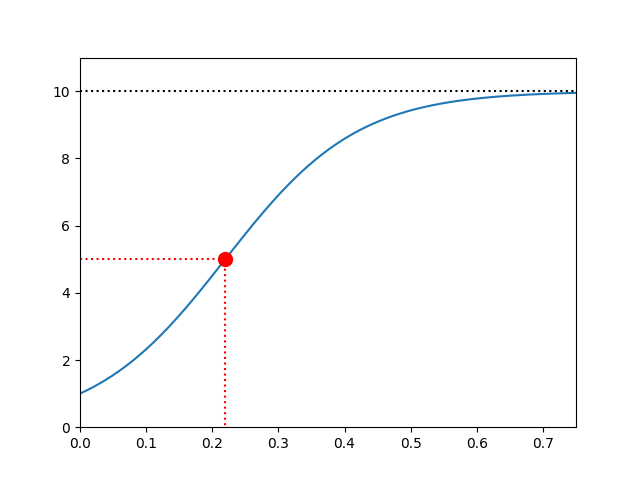
This equation \eqref{eq:ode-sol-logistic-fcn} is called logistic function or logistic equation and it comes in lots and lots of fields such as ecology, statistics and machine learning (hence AI), medicine, chemistry, physics, material science, linguistics, agriculture, economics and sociology, etc. For more information, please refer to Logistic function Wikipedia Page.
There are several things we can observe from this function!
- as long as $0< y(0) < b$, $y(t)$ monotonically increases (because $y’(t)>0$ for $t>0$)
- $\lim_{t\to\infty} y(t) = b$
- $y(t)$ is concave up (i.e., $y$ is a convex function) where $y(t) < b/2$
- $y(t)$ is concave down (i.e., $y$ is a concave function) where $y(t) > b/2$
- $y(t)$ reaches its middle point at $t = - C/ab$, i.e., $y(-C/ab) = b/2$ (thus, if $C>0$, $y(t)$ is always concave down)
The graph below shows $y(t)$ when $a=1$, $b=10$, and $y(0)=1$. The calculation shows it reaches its middle point at $t \simeq 0.21972$ We can see indeed the graph is concave up where $t< 0.21972$ and is concave down where $t>0.21972$!
Interactive animation — watch the solution evolve in real time
Exercise Problems
Differentiation & Integration
-
Varsity Tutors Problem
Evaluate $f'(1)$ when $f(x) = \int_0^x (6t^2 - 3t + 10) dt$.
Answer $$ 13 $$
-
Varsity Tutors Problem
Evaluate:
$$
\int_0^{\infty} \frac{\cos x}{e^x} dx
$$
Answer $$ \frac{1}{2} $$
-
Varsity Tutors Problem
Evaluate:
$$
\int_0^{\infty} \frac{x}{e^{x^2}} dx
$$
Answer $$ \frac{1}{2} $$
-
Varsity Tutors Problem
Evaluate:
$$
\int_0^{\infty} \frac{\cos x}{e^{x^2}} dx
$$
Answer $$ \frac{1}{2} $$
-
Varsity Tutors Problem
Find $\frac{dy}{dx}$ if $x^3-x\ln y=ye^x$.
Answer $$ \frac{dy}{dx} = \frac{3x^2y-y\ln y - y^2 e^x}{e^x y+x} $$
-
Varsity Tutors Problem
Find $dy/dx$:
$$
y = \tan^{-1} (2x(x+1)^{10}))
$$
Answer $$ \frac{dy}{dx} = \frac{2(x+1)^9 (11x+1)}{1+4x^2(x+1)^{20}} $$
-
Varsity Tutors Problem
What is the derivative of $r=7\sin\theta -6$?
Answer $$ \frac{dy}{dx} = \frac{7\sin 2\theta - 6 \cos\theta}{7\cos 2\theta + 6\sin\theta} = \frac{14\cos\theta \sin\theta - 6 \cos\theta}{7 - 14\sin^2\theta + 6\sin\theta} $$
-
Varsity Tutors Problem
Let $f(x) = \cos(4x)$ on the interval $(0,\pi/2)$.
Find a value for the number(s) that
satisfies the [mean value theorem](#mean-value-theorem)
for this function and interval.
Answer $$ \frac{\pi}{4} $$
-
Varsity Tutors Problem
Approximate
$$
\int_1^2 x^2 \ln x \, dx
$$
using the midpoint rule with $n=5$. Round your answer to three decimal places.
Answer $$ 1.064 $$
-
Varsity Tutors Problem
Approximate
$$
\int_0^{\pi/4} \tan^2 x \, dx
$$
using the trapezoidal rule with $n=4$. Round your answer to three decimal places.
Answer $$ 0.227 $$
-
Varsity Tutors Problem
Given
$$
f(x) = \int_0^x \left( \frac{1}{t^2} - 2t + 3\right) dt
$$
what is $f'(6)$?
- $\frac{323}{36}$
- $-\frac{36}{323}$
- $-\frac{323}{36}$
- $\frac{36}{323}$
- None of the above.
Answer 3.
-
Varsity Tutors Problem
Evaluate
$$
\int_1^\infty \frac{4}{x^5} dx
$$
- $-\infty$
- $0$
- $1$
- $-1$
- $\infty$
Answer 3.
-
Varsity Tutors Problem
$$
\int \frac{x-1}{(x-3)(x+4)} dx =
$$
- $\frac{5}{7(x+4)} \ln |x| + \frac{2}{7(x-3)} \ln |x| + C$
- $\frac{1}{7} \ln |x-2| + \frac{1}{7} \ln |x-4| + C$
- $\frac{5}{7(x+4)} + \frac{2}{7(x+2)} + C$
- $\frac{2}{7} \ln |x-3| + \frac{5}{7} \ln |x+4| + C$
- $\frac{(x-3)^2}{7} + \frac{2(x+4)^2}{7} + C$
Answer 4.
Length & Distance & Velocity & Acceleration & Energy
-
Varsity Tutors Problem Given the velocity function
$$
v(t) = \int_0^{t^2+2t+1} z^d \sin(z^5)\,dz
$$
where $d$ is real number such that $d\in(0,1)$,
find the acceleration function $a(x)$
Daddy's Solution We use the first part of FTC i.e., \eqref{eq:fund-theorem-of-calculus-1} to get $$ \begin{eqnarray*} a(t) &=& \frac{d}{dt} v(t) = (2t+2) (t^2+2t+1)^d \sin((t^2+2t+1)^5) \\ &=& 2(t+1)^{2d+1} \sin((t+1)^{10}) \end{eqnarray*} $$ by noting that $t^2+2t+1=(t+1)^2$. -
Varsity Tutors Problem
Given $\vec{r}(t) = (5t^3, e^{11t}, e^{5t})$.
Calculate $\dfrac{d}{dt} \vec{r}(t)$.
Answer $$ \frac{d}{dt} \vec{r}(t) = (15t^2, 11e^{11t}, 5e^{5t}) $$
-
Varsity Tutors Problem
Find the equation for the velocity of a particle if the acceleration of the particle is given by
$$
a(t) = 16 t^2 + 48
$$
and the velocity at time $t=0$ of the particle is $30$.
Answer $$ v(t) = \frac{16}{3} t^3 + 48 t + 30 $$
-
Varsity Tutors Problem
What is the length of the curve $g(x) = x^{3/2}$ over the interval $0\leq x\leq 4$?
Daddy's Solution $$ \begin{eqnarray*} \int_{0}^4 \sqrt{1+g'(x)^2}\, dx &=& \int_{0}^4 \sqrt{1+\frac{9}{4}x} \,dx \\ &=& \frac{4}{9} \cdot \frac{2}{3} \left.\left(1+\frac{9}{4}x\right)^{3/2}\right|_{x=0}^4 \\ &=& \frac{8}{27} (10\sqrt{10}-1) \end{eqnarray*} $$
-
Varsity Tutors Problem Given $x=t+10$ and $y=2t-9$,
what is the arc length between $0\leq t\leq 4$?
Answer $$ 4\sqrt{5} $$
-
Varsity Tutors Problem
Find the length of the following parametric curve
$$
x = e^t \cos(t),\;
y = e^t \sin(t),\;
0 \leq t \leq 2\pi.
$$
- $\sin(t)+\cos(t)$
- $e^t \cos(t)$
- $1$
- $e^{2\pi}$
- $\sqrt{2} (e^{2\pi} -1)$
Daddy's Solution Note first that the length of the curve can be calculated by $$ \int_0^{2\pi} |\vec{v}(t)| dt $$ by \eqref{eq:vel-int-len} where $\vec{v}(t)$ is the velocity vector. Now the displacement (i.e., location) vector is given by $$ \vec{d}(t) = (x(t), y(t)) = (e^t \cos t, e^t \sin t) $$ hence the velocity vector can be calculated as $$ \vec{v}(t) = \frac{d}{dt} \vec{d}(t) = \left( \frac{d}{t} x(t), \frac{d}{dt} y(t) \right) = (e^t(\cos t - \sin t), e^t (\sin t + \cos t)) $$ and the size of $\vec{v}(t)$ is $$ \begin{eqnarray*} |\vec{v}(t)| &=& e^t \sqrt{(\cos t - \sin t)^2 + (\cos t + \sin t)^2} \\ &=& e^t \sqrt{(\cos t - \sin t)^2 + (\cos t + \sin t)^2} \\ &=& \sqrt{2}\, e^t \end{eqnarray*} $$ Therefore the length can be calculated as $$ \int_0^{2\pi} |\vec{v}(t)| dt = \sqrt{2} \int_0^{2\pi} e^t dt = \sqrt{2} \, \left.\left( e^t \right)\right|_{t=0}^{2\pi} = \sqrt{2} (e^{2\pi} -1) $$ -
Varsity Tutors Problem
The temperature of an oven is increasing at a rate $r(t) = 2 e^{0.5 t}$
degrees Fahrenheit per miniute for $0\leq t\leq 10$ minutes.
The initial temperature of the oven is $T(0) = 75$ degrees Fahrenheit.
What is the temperture of the oven at $t = 5$? Round your answer to the nearest tenth.
- 119.7
- 212.2
- 239.4
- 323.9
Answer 1.
-
Varsity Tutors Problem
Give the arclength of the graph of the function $f(x) = \frac{1}{2} \ln(\cos 2x)$
on the interval $[0, \frac{\pi}{8}]$.
- $\frac{1}{2} \ln\left(1+\sqrt{2}\right)$
- $1+\sqrt{2}$
- $\frac{1}{2} + \frac{1}{2} \sqrt{2}$
- $\frac{1}{2} + \frac{1}{2} \ln{2}$
- $\ln\left(1+\sqrt{2}\right)$
Answer 1.
Area & Volume
-
Varsity Tutors Problem
Find the volume of the solid generated by rotating about the $y$-axis the region under the curve $y=\sqrt{x}$,
from $0$ to $4$.
- $\frac{64}{3} \pi$
- $\frac{256}{7} \pi^2$
- $\frac{128}{5} \pi$
- $\frac{\pi}{2}$
- None of the other answers
Answer 3.
Polar Coordinates
- Varsity Tutors Problem What is the polar form of $y=-7x^2$?
Answer $$ r(\theta) = - \frac{\sin\theta}{7\cos^2\theta} = - \frac{1}{7} \tan\theta \sec\theta $$
Taylor Series and Approximation
-
Varsity Tutors Problem
Write out the first three terms of the Taylor series about $a=1$ for the following function.
$$
f(x) = x^2 + e^x
$$
Answer $$ \begin{eqnarray*} f(x) &\simeq& f(1) + f'(1) (x-1) + \frac{1}{2!} f^{\prime\prime}(x) (x-1)^2 \\ &=& 1 + e + (2+e)(x-1) + \frac{1}{2} (2+e)(x-1)^2 \end{eqnarray*} $$
-
Varsity Tutors Problem
Write the first three terms of the Taylor series for the following function about $x=1$:
$$
f(x) = x^2 + 3x + 2
$$
Answer $$ \begin{eqnarray*} f(x) &\simeq& f(1) + f'(1) (x-1) + \frac{1}{2!} f^{\prime\prime}(x) (x-1)^2 \\ &=& 6 + 5(x-1) + (x-1)^2 \end{eqnarray*} $$
-
Varsity Tutors Problem
For which of the following functions can the Maclaurin series representation be expressed in four or fewer non-zero terms?
- $f(x) = x^5/3+2$
- $f(x) = x^2 + \sqrt{x} + 1$
- $f(x) = \ln |x + 3|$
- $f(x) = x + 3 \sin(x)$
Answer 1.
-
Varsity Tutors Problem
Write out the first three terms of the Taylor series about $a=1$ for the following function:
$$
f(x) = 10x^2 + x
$$
- $11+21x+10x^2$
- $11+21(x-1)+10(x-1)^2$
- $0 + 0 + 0$
- $0 + 21(x-1) + 10(x-1)^2$
Answer 2.
-
Varsity Tutors Problem
Write out the first four terms of the Taylor series about $a=1$ for the following function:
$$
f(x) = x^2+2x+1
$$
- $0 + 0 + 0 + 0$
- $0 + 4 + 4(x-1) + (x-1)^2$
- $4 + 4(x-1) + (x-1)^2 + 0$
- $4 + 4(x-1)^2 + (x-1)^3 + 0$
Answer 3.
Infinite Sequences and Series
-
Varsity Tutors Problem
Calculate the sum of a geometric series with the following values:
$$
n=10,\;
a_1 = 11,\;
r = \frac{2}{20}
$$
rounded to the nearest integer.
Answer $$ 12 $$
-
Varsity Tutors Problem
For the series $\sum_{n=0}^\infty (-1)^n (\frac{n^n}{8^n})$,
determine if the series converge or diverge.
If it diverges, choose the best reason.
Answer The series diverges, since $\lim_{n\to\infty} x_n \neq0$.
-
Varsity Tutors Problem
Determine whether the series converges or diverges:
$$
\sum_{n=1}^\infty (-1)^{n+1} \frac{n^4}{2n^4+1}
$$
- The series may be convergent, divergent, or conditionally convergent.
- The series is conditionally convergent.
- The series is (absolutely) convergent.
- The series is divergent.
Answer 4.
-
Varsity Tutors Problem
Determine if the series converges or diverges. You do not need to find the sum.
$$
\sum_{n=1}^\infty \frac{1}{n^3+2}
$$
Answer The series converges.
-
Varsity Tutors Problem
Find the interval of convergence of $x$ for the series
$$
\sum_{n=1}^\infty \frac{3^n x^n}{n!}
$$
Answer $$ (-\infty, \infty) $$
-
Varsity Tutors Problem
Which of the following series does not converge?
- $\sum_{i=0}^\infty \frac{n!}{n^2\cos(n)}$
- $\sum_{i=0}^\infty \frac{n-1}{n^3+1}$
- $\sum_{i=0}^\infty 0.9999999999999999999^n$
- $\sum_{i=0}^\infty \frac{(-1)^n}{n}$
- $\sum_{i=0}^\infty \frac{n^2 \ln(n)}{n!}$
Answer 1.
-
Varsity Tutors Problem
Which of following intervals of convergence cannot exist?
- $[2,\infty)$
- For any $q$, $p$ such that $q\leq p$, the interval $[q,p]$
- $[2,10000)$
- For any $\epsilon >0$, the interval $[a-\epsilon,a+\epsilon]$ for some $a\in\reals$
Answer 1.
-
Varsity Tutors Problem
Determine whether
$$
\sum_{n=1}^\infty (-1)^n \sin (1/n)
$$
converges or diverges, and explain why.
Answer The series (conditionally) converges, which can be confirmed by the alternating series test.
-
Varsity Tutors Problem
Determine whether the following series converges or diverges:
$$
\sum_{n=0}^\infty (-1)^n \left(\frac{5}{n}\right)
$$
Answer The series (conditionally) converges, which can be confirmed by the alternating series test.
-
Varsity Tutors Problem
One of the following infinite series converges. Which is it?
- $\sum_{k=1}^\infty \frac{1}{k}$
- $\sum_{k=1}^\infty \frac{\sin(k)}{k^2}$
- $\sum_{k=1}^\infty (-1)^k \sin(k)$
- $\sum_{k=2}^\infty \frac{k}{\ln(k)}$
- None of the others converge.
Answer 2.
-
Varsity Tutors Problem
Determine whether the following series converges or diverges. If it converges, what does it converge to?
$$
\sum_{n=0}^\infty (2)^{-2n}
$$
- $\dfrac{3}{4}$
- Diverges
- $1$
- $\dfrac{4}{3}$
Answer 4.
-
Varsity Tutors Problem
Determine the nature of convergence of the series having the general term:
$$
\frac{8}{\sqrt{n(n+1)(n+2)}}
$$
- $\frac{\pi}{7}$
- $\frac{\pi}{5}$
- The series is convergent.
- $\frac{1}{2}$
- The series is divergent.
Answer 3.
-
Varsity Tutors Problem
Determine if the following series is divergent, convergent or neither.
$$
\sum_{n=1}^\infty \frac{n!}{2^{n+1}}
$$
- Neither
- Inconclusive
- Both
- Divergent
- Convergent
Answer 4.
Differential Equations
-
Problem 4 of AP Calculus (BC) Chapter 6 Test
–
Given the logistic differential equation $\dfrac{dA}{dt} = A\left(20-\dfrac{A}{4}\right)$
where $A(0) = 15$, what is $\lim_{t\to\infty} A(t)$?
Daddy's Solution 1 $$ \begin{eqnarray*} \frac{dA}{A(20-A/4)} = dt &\Leftrightarrow& \left( \frac{1}{A} + \frac{1}{80-A} \right) dA = 20dt \\ &\Leftrightarrow& \ln A - \ln (80 - A) = 20 t + C \\ &\Leftrightarrow& \ln \left( \frac{A}{80 - A} \right) = 20 t + C \\ &\Leftrightarrow& \ln \left( \frac{1}{80/A - 1} \right) = 20 t + C \\ &\Leftrightarrow& \ln ( 80/A - 1 ) = -20 t - C \\ &\Leftrightarrow& 80/A = e^{-20 t - C} + 1 \\ &\Leftrightarrow& A = \frac{80}{e^{-20 t - C} + 1} \end{eqnarray*} $$Daddy's Solution 2 Let's try to solve using the formula we derived above, i.e., \eqref{eq:ode-sol-logistic-fcn}! Because we can rewrite the logistic differential equation as $$ \frac{dA}{dt} = \frac{1}{4} A(80-A) $$ and this equation is of the form \eqref{eq:ode-logistic-fcn} with $a=1/4$ and $b=80$, the formula \eqref{eq:ode-sol-logistic-fcn} gives $$ A(t) = \frac{80}{1+ e^{-20t-C}} $$
-
Problem 13 of AP Calculus (BC) Chapter 6 Test
$$
\frac{dP}{dt} = \frac{k}{656} (650- P) P, \; P(0) = 1
$$
Daddy's Solution Note that the above equation is of the form \eqref{eq:ode-logistic-fcn} with $a=k/650$ and $b=650$, thus the formula \eqref{eq:ode-sol-logistic-fcn} gives $$ P(t) = \frac{650}{1+e^{-kt-C}} = \frac{650}{1+C' e^{-kt}} $$ thus of the same form as in the problem! -
Problem 5 of AP Calculus (BC) Chapter 6 Test
–
Given the differential equation $\dfrac{dT}{dt} = -\dfrac{1}{4}(T-20)$, $T(0)=100$, then $T(20)$?
Daddy's Solution 1 $$ \begin{eqnarray*} \frac{dT}{T-20} = -\frac{1}{4} dt &\Leftrightarrow& \ln (T-20) = -\frac{1}{4} t + C \\ &\Leftrightarrow& T(t) = 20 + e^{-\frac{1}{4} t + C} \end{eqnarray*} $$ If we use $T(0)=100$, we have $$ \ln(80) = C $$ hence $$ T(t) = 20 + e^{-\frac{1}{4} t + \ln(80)} = 20 + 80 e^{-\frac{1}{4}t} $$Daddy's Solution 2 Let's try to solve using the formula we derived above, i.e., \eqref{eq:ode-linear-sol}. Because we can rewrite the differential equation as $$ \frac{dT}{dt} = - \frac{1}{4} T + 5 $$ and this equation is of the form \eqref{eq:ode-linear} with $a=-1/4$ and $b=5$, the formula \eqref{eq:ode-linear-sol} gives $$ T(t) = (100 - 20) e^{-\frac{1}{4}t} + 20 $$
Exercise Problem Collection
Area and Volume
- c_11.1_ca1.pdf
- c_11.1_ca2.pdf
- c_11.1_packet.pdf
- c_11.1_solutions.pdf
- c_11.2_ca1.pdf
- c_11.2_ca2.pdf
- c_11.2_packet.pdf
- c_11.2_solutions.pdf
- c_11.3_ca1.pdf
- c_11.3_ca2.pdf
- c_11.3_packet.pdf
- c_11.3_solutions.pdf
- c_11.4_ca1.pdf
- c_11.4_ca2.pdf
- c_11.4_packet.pdf
- c_11.4_solutions.pdf
- c_11_review_solutions.pdf
- c_11_review.pdf
- free_response_on_area_and_volume.pdf
- free_response_answers_on_area_and_volume.pdf
Appendix
Some trigonometric equivalences
Pythagorean Identities
\begin{equation} \label{eq:tri-pythagorean-identity} \sin^2 \theta + \cos^2 \theta = 1 \end{equation}
which implies
\begin{equation} \label{eq:tri-pythagorean-identity-sin} \sin \theta = \pm \sqrt{1-\cos^2\theta} \end{equation}
\begin{equation} \label{eq:tri-pythagorean-identity-cos} \cos \theta = \pm \sqrt{1-\sin^2\theta} \end{equation}
\begin{equation} \label{eq:tri-pythagorean-identity-csc} 1 + \cot^2\theta = \csc^2 \theta \end{equation}
\begin{equation} \label{eq:tri-pythagorean-identity-sec} 1 + \tan^2\theta = \sec^2 \theta \end{equation}
\begin{equation} \label{eq:tri-pythagorean-identity-sec-csc} \sec^2\theta + \csc^2\theta = \sec^2 \theta \csc^2\theta \end{equation}
Shifts and Periodicity
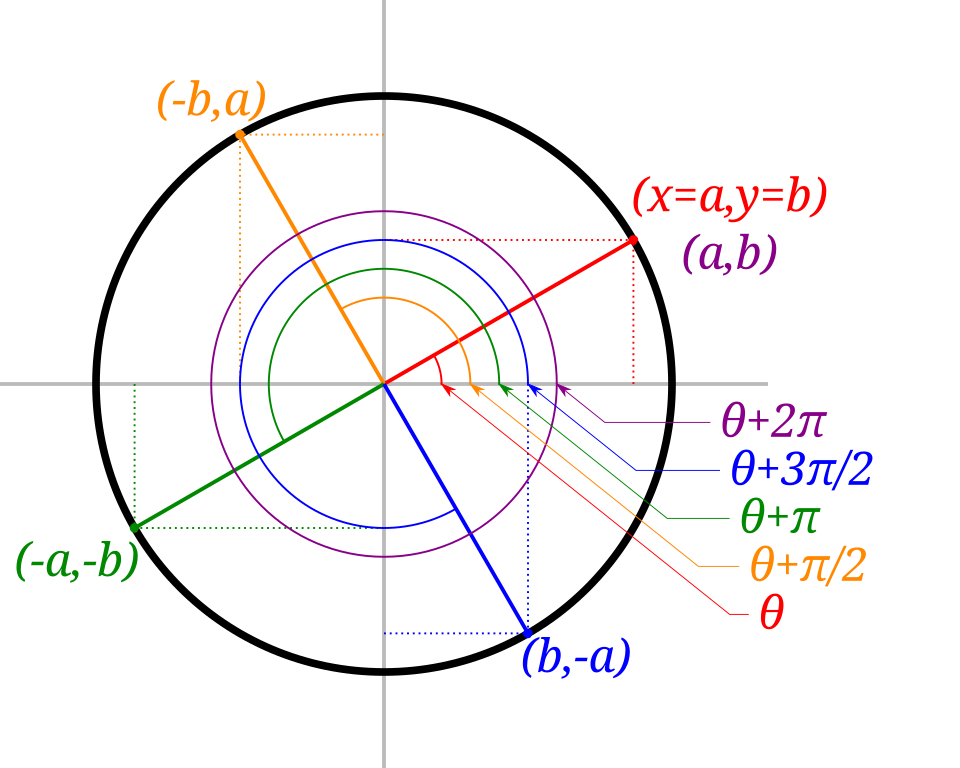
| function | period | shift by $\dfrac{\pi}{2}$ | shift by $\pi$ | shift by multiples of $2\pi$ |
| $\sin$ | $2\pi$ | $\sin\left(\theta \pm \dfrac{\pi}{2}\right) = \pm \cos\theta$ | $\sin(\theta+\pi) = - \sin\theta$ | $\sin(\theta + k\cdot 2\pi) = + \sin\theta$ |
| $\cos$ | $2\pi$ | $\cos\left(\theta \pm \dfrac{\pi}{2}\right) = \mp \sin\theta$ | $\cos(\theta+\pi) = - \cos\theta$ | $\cos(\theta + k\cdot 2\pi) = + \cos\theta$ |
| $\tan$ | $\pi$ | $\tan\left(\theta \pm \dfrac{\pi}{2}\right) = - \cot\theta$ | $\tan(\theta+\pi) = + \tan\theta$ | $\tan(\theta + k\cdot 2\pi) = + \tan\theta$ |
| $\csc$ | $2\pi$ | $\csc\left(\theta \pm \dfrac{\pi}{2}\right) = \pm \sec\theta$ | $\csc(\theta+\pi) = - \csc\theta$ | $\csc(\theta + k\cdot 2\pi) = + \csc\theta$ |
| $\sec$ | $2\pi$ | $\sec\left(\theta \pm \dfrac{\pi}{2}\right) = \mp \csc\theta$ | $\sec(\theta+\pi) = - \sec\theta$ | $\sec(\theta + k\cdot 2\pi) = + \sec\theta$ |
| $\cot$ | $\pi$ | $\cot\left(\theta \pm \dfrac{\pi}{2}\right) = - \tan\theta$ | $\cot(\theta+\pi) = + \cot\theta$ | $\cot(\theta + k\cdot 2\pi) = + \tan\theta$ |
| function | shift by $\dfrac{\pi}{4}$ | shift by $\dfrac{\pi}{2}$ | shift by multiples of $\pi$ |
| $\tan$ | $\tan\left(\theta \pm \dfrac{\pi}{4}\right) = \dfrac{\tan\theta \pm 1}{1 \mp \tan \theta}$ | $\tan\left(\theta + \dfrac{\pi}{2}\right) = - \cot\theta$ | $\tan(\theta + k\cdot \pi) = + \tan\theta$ |
| $\cot$ | $\cot\left(\theta \pm \dfrac{\pi}{4}\right) = \dfrac{\cot\theta \mp 1}{1 \pm \cot \theta}$ | $\cot\left(\theta + \dfrac{\pi}{2}\right) = - \tan\theta$ | $\cot(\theta + k\cdot \pi) = + \cot\theta$ |
Reflections, Shifts, and Periodicity
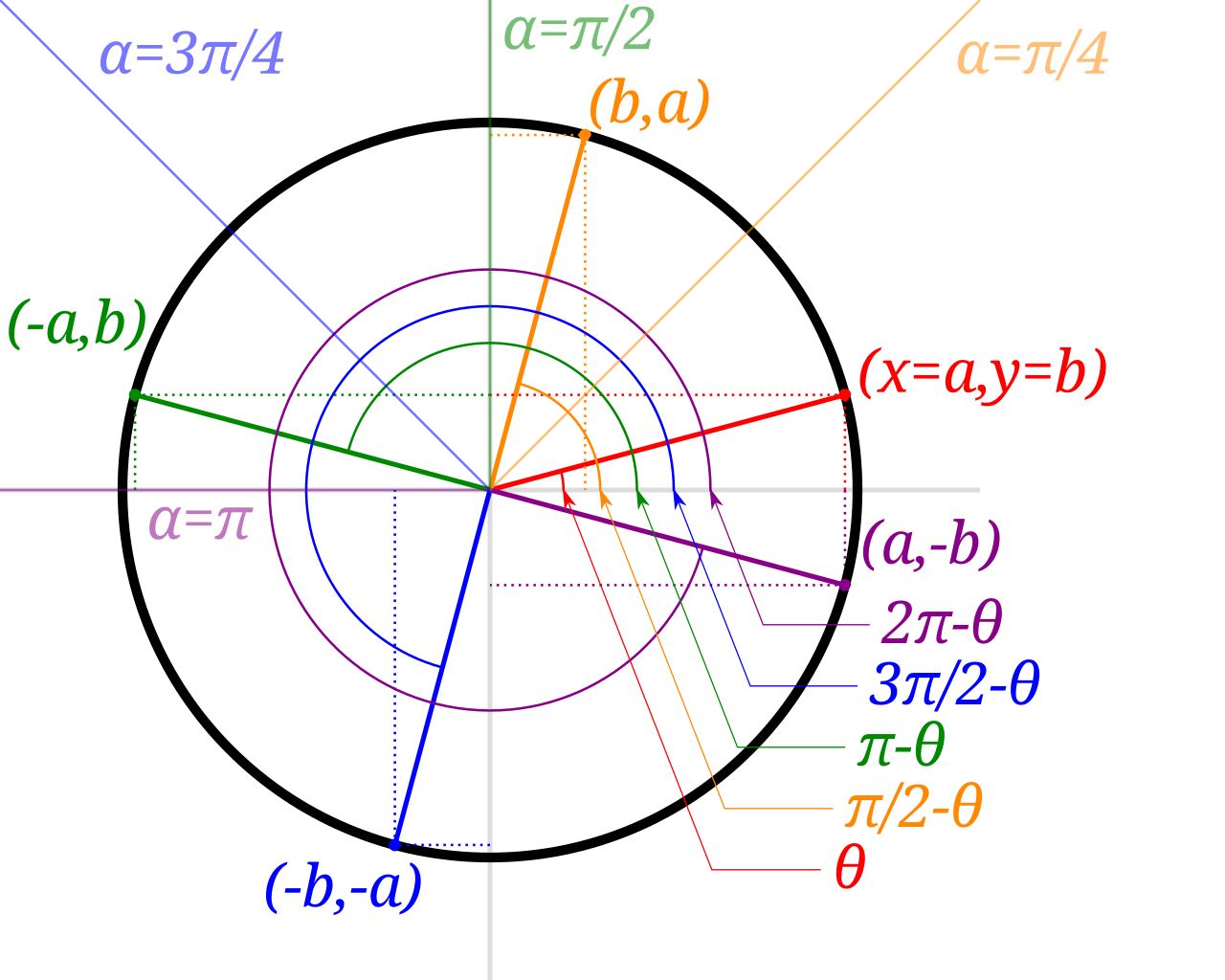
| $\theta$ reflected in $\alpha=0$ | $\theta$ reflected in $\alpha=\dfrac{\pi}{4}$ | $\theta$ reflected in $\alpha=\dfrac{\pi}{2}$ | $\theta$ reflected in $\alpha=\dfrac{3\pi}{4}$ | $\theta$ reflected in $\alpha=\pi$ |
| $\sin(-\theta) = - \sin\theta$ | $\sin\left(\dfrac{\pi}{2}-\theta\right) = + \cos\theta$ | $\sin(\pi-\theta) = + \sin\theta$ | $\sin\left(\dfrac{3\pi}{2}-\theta\right) = - \cos\theta$ | $\sin(2\pi-\theta) = \sin(-\theta) = - \sin \theta$ |
| $\cos(-\theta) = + \cos\theta$ | $\cos\left(\dfrac{\pi}{2}-\theta\right) = + \sin\theta$ | $\cos(\pi-\theta) = - \cos\theta$ | $\cos\left(\dfrac{3\pi}{2}-\theta\right) = - \sin\theta$ | $\cos(2\pi-\theta) = \cos(-\theta) = + \cos \theta$ |
| $\tan(-\theta) = - \tan\theta$ | $\tan\left(\dfrac{\pi}{2}-\theta\right) = + \cot\theta$ | $\tan(\pi-\theta) = - \tan\theta$ | $\tan\left(\dfrac{3\pi}{2}-\theta\right) = + \cot\theta$ | $\tan(2\pi-\theta) = \tan(-\theta) = - \tan \theta$ |
| $\csc(-\theta) = - \csc\theta$ | $\csc\left(\dfrac{\pi}{2}-\theta\right) = + \sec\theta$ | $\csc(\pi-\theta) = + \csc\theta$ | $\csc\left(\dfrac{3\pi}{2}-\theta\right) = - \sec\theta$ | $\csc(2\pi-\theta) = \csc(-\theta) = - \csc \theta$ |
| $\sec(-\theta) = + \sec\theta$ | $\sec\left(\dfrac{\pi}{2}-\theta\right) = + \csc\theta$ | $\sec(\pi-\theta) = - \sec\theta$ | $\sec\left(\dfrac{3\pi}{2}-\theta\right) = - \csc\theta$ | $\sec(2\pi-\theta) = \sec(-\theta) = + \sec \theta$ |
| $\cot(-\theta) = - \cot\theta$ | $\cot\left(\dfrac{\pi}{2}-\theta\right) = + \tan\theta$ | $\cot(\pi-\theta) = - \cot\theta$ | $\cot\left(\dfrac{3\pi}{2}-\theta\right) = + \tan\theta$ | $\cot(2\pi-\theta) = \cot(-\theta) = - \cot \theta$ |
Sum and Difference Identities
\[\begin{eqnarray} \label{eq:tri-sin-sum-identity} \sin(\alpha + \beta) &=& \sin\alpha \cos\beta + \cos\alpha \sin\beta \\ \label{eq:tri-cos-sum-identity} \cos(\alpha + \beta) &=& \cos\alpha \cos\beta - \sin\alpha \sin\beta \end{eqnarray}\]hence
\[\begin{eqnarray} \sin(\alpha - \beta) &=& \sin\alpha \cos\beta - \cos\alpha \sin\beta \\ \cos(\alpha - \beta) &=& \cos\alpha \cos\beta + \sin\alpha \sin\beta \end{eqnarray}\]which imply
\[\begin{eqnarray} \tan(\alpha + \beta) &=& \frac{\tan\alpha + \tan \beta}{1 - \tan\alpha\tan\beta} \\ \tan(\alpha - \beta) &=& \frac{\tan\alpha - \tan \beta}{1 + \tan\alpha\tan\beta} \end{eqnarray}\]Multiple-angle Formulas
We can derive all the formula here essentially using these two formulas; \eqref{eq:tri-sin-sum-identity} and \eqref{eq:tri-cos-sum-identity}!
- \eqref{eq:tri-sin-sum-identity} implies \begin{equation} \label{eq:tri-sin-2-theta} \sin(2\theta) = 2\sin\theta \cos\theta \end{equation}
- \eqref{eq:tri-cos-sum-identity} (together with \eqref{eq:tri-pythagorean-identity}) implies \begin{equation} \label{eq:tri-cos-2-theta} \cos(2\theta) = \cos^2 \theta - \sin^2\theta = 1 - 2\sin^2\theta = 2\cos^2\theta - 1 \end{equation}
- \eqref{eq:tri-sin-2-theta} and \eqref{eq:tri-cos-2-theta} imply \begin{equation} \label{eq:tri-tan-2-theta} \tan(2\theta) = \frac{2\tan\theta}{1 - \tan^2\theta} \end{equation}
- \eqref{eq:tri-sin-sum-identity}, \eqref{eq:tri-sin-2-theta}, and \eqref{eq:tri-cos-2-theta} (together with \eqref{eq:tri-pythagorean-identity}) imply \begin{equation} \label{eq:tri-sin-3-theta} \sin(3\theta) = 3\sin\theta - 4\sin^3\theta \end{equation} because $$ \begin{eqnarray*} \sin(3\theta) &=& \sin(\theta + 2\theta) = \sin\theta \cos(2\theta) + \cos\theta \sin(2\theta) \\ &=& \sin\theta (1-2\sin^2\theta) + 2\cos^2\theta \sin\theta \\ &=& \sin\theta (1-2\sin^2\theta) + 2(1-\sin^2\theta) \sin\theta \\ &=& 3\sin\theta - 4\sin^3\theta \end{eqnarray*} $$
- \eqref{eq:tri-sin-3-theta} implies \begin{equation} \label{eq:tri-cos-3-theta} \cos(3\theta) = -3\cos\theta + 4\cos^3\theta \end{equation} because $$ \begin{eqnarray*} \cos(3\theta) &=& - \sin \left(3\theta + \frac{3\pi}{2} \right) = - \sin \left(3\left(\theta + \frac{\pi}{2}\right) \right) \\ &=& - 3\sin\left(\theta + \frac{\pi}{2}\right) + 4\sin^3\left(\theta + \frac{\pi}{2}\right) \\ &=& - 3\cos\theta + 4\cos^3\theta \end{eqnarray*} $$
- Now \eqref{eq:tri-sin-3-theta}, \eqref{eq:tri-cos-3-theta}, and \eqref{eq:tri-pythagorean-identity-sec} imply \begin{equation} \label{eq:tri-tan-3-theta} \tan(3\theta) = \frac{3\tan\theta - \tan^3\theta}{1 - 3\tan^2\theta} \end{equation} because $$ \begin{eqnarray*} \tan(3\theta) &=& \frac{3\sin\theta - 4\sin^3\theta}{-3\cos\theta + 4\cos^3\theta} = \frac{3\tan\theta \sec^2\theta - 4\tan^3\theta}{-3\sec^2\theta + 4} \\ &=& \frac{3\tan\theta (1+\tan^2\theta) - 4\tan^3\theta}{-3(1+\tan^2\theta) + 4} \\ &=& \frac{3\tan\theta - \tan^3\theta}{1 - 3\tan^2\theta} \end{eqnarray*} $$
Half-angle formulas
Similarly, all the formulas here can be (easily) derived from what we have studied so far.
- \eqref{eq:tri-cos-2-theta} readily implies \begin{equation} \label{eq:tri-sin-half-theta} \sin^2\frac{\theta}{2} = \frac{1-\cos\theta}{2} \end{equation}
- Also, \eqref{eq:tri-cos-2-theta} readily implies \begin{equation} \label{eq:tri-cos-half-theta} \cos^2\frac{\theta}{2} = \frac{1+\cos\theta}{2} \end{equation}
- Now \eqref{eq:tri-sin-2-theta}, \eqref{eq:tri-sin-half-theta}, and \eqref{eq:tri-cos-half-theta}, imply \begin{equation} \label{eq:tri-tan-half-theta} \tan\frac{\theta}{2} = \frac{1-\cos\theta}{\sin\theta} = \frac{\sin\theta}{1+\cos\theta} = \frac{\tan\theta}{1+\sec\theta} \end{equation} because $$ \begin{eqnarray*} \tan\frac{\theta}{2} &=& \frac{\sin(\theta/2)}{\cos(\theta/2)} \\ &=& \frac{2\sin^2(\theta/2)}{2\sin(\theta/2)\cos(\theta/2)} = \frac{1-\cos\theta}{\sin\theta} \\ &=& \frac{2\cos(\theta/2)\sin(\theta/2)}{2\cos^2(\theta/2)} = \frac{\sin\theta}{1+\cos\theta} = \frac{\tan\theta}{\sec\theta+1} \end{eqnarray*} $$
Power-reduction formulas
Once again, everything here can be deduced from what we’ve already studied!3
So in a sense, essentially, no addition knowledge adds up here, but it’s always good to know and get accustomed to these patterns, e.g., to get good grades on AP Calculus BC tests! ★^^★
- \eqref{eq:tri-cos-2-theta} implies \begin{equation} \label{eq:tri-sin-squared} \sin^2\theta = \frac{1 - \cos(2\theta)}{2} \end{equation} \begin{equation} \label{eq:tri-cos-squared} \cos^2\theta = \frac{1 + \cos(2\theta)}{2} \end{equation}
- \eqref{eq:tri-sin-3-theta} and \eqref{eq:tri-cos-3-theta} respectively imply \begin{equation} \label{eq:tri-sin-cubed} \sin^3\theta = \frac{3\sin\theta - \sin(3\theta)}{4} \end{equation} \begin{equation} \label{eq:tri-cos-cubed} \cos^3\theta = \frac{3\cos\theta + \cos(3\theta)}{4} \end{equation}
- Some (tedious) calculations also lead to \begin{equation} \label{eq:tri-sin-power-4} \sin^4\theta = \frac{3 - 4\cos(2\theta) + \cos(4\theta)}{8} \end{equation} \begin{equation} \label{eq:tri-cos-power-4} \cos^4\theta = \frac{3 + 4\cos(2\theta) + \cos(4\theta)}{8} \end{equation} \begin{equation} \label{eq:tri-sin-power-5} \sin^5\theta = \frac{10\sin\theta - 5\sin(3\theta) + \sin(5\theta)}{16} \end{equation} \begin{equation} \label{eq:tri-cos-power-5} \cos^5\theta = \frac{10\cos\theta + 5\cos(3\theta) + \cos(5\theta)}{16} \end{equation}
Interactive Visualization Tools
Power Functions
Drag the slider to sweep $p$ continuously from $-3$ to $3$. The tool draws $f(x) = x^p$ and its derivative $f’(x) = p\,x^{p-1}$ live for $x \ge 0$, so you can watch the geometry morph in real time — and see exactly how the derivative rule works across every case – integer, fractional, negative, and zero exponents!
Antiderivative of Power Functions
This is the flip side of the previous tool — now we look at $f(x) = \dfrac{x^p}{p}$ and its derivative $f’(x) = x^{p-1}$. This is exactly the power rule for integration!
\[\int x^{p-1}\,dx = \frac{x^p}{p} + C \quad \mbox{for }p \neq 0\]Drag $p$ and notice the beautiful symmetry with the previous tool – the derivative of $\displaystyle \frac{x^p}{p}$ is always $x^{p-1}$ — watch how $f’(x) = x^{p-1}$ changes shape as $p$ sweeps, and observe the special cases carefully!
- What happens at $p=1$?
- What happens at $p=0.5$?
- What happens at $p=0$ (the famous exception where $\displaystyle \int x^{-1} dx = \ln x$, not a power function!)?
- For example, for every trigonometric differentiation formulas can be derived from this single formula! $$ \frac{d}{dx} \sin x = \cos x $$ *i.e.*, we can even derive the derivative of the cosine function from this by $$ \frac{d}{dx} \cos x = \frac{d}{dx} \sin \left(x + \frac{\pi}{2}\right) = \cos \left(x + \frac{\pi}{2}\right) \frac{d}{dx} \left(x + \frac{\pi}{2}\right) = - \sin x $$ where the chain rule \eqref{eq:chain-rule} is used! ↩
- The notion of a sequence can be generalized to an indexed family, defined as a function from an arbitrary index set. ↩
- Indeed, we do NOT even need both \eqref{eq:tri-sin-sum-identity} and \eqref{eq:tri-cos-sum-identity}, because one readily implies the other. For example, assume that we only knew \eqref{eq:tri-sin-sum-identity}. Then we can derive $$ \begin{eqnarray*} \cos(\alpha + \beta) &=& \sin\left(\alpha + \beta + \frac{\pi}{2}\right) = \sin\left(\alpha + \left(\beta + \frac{\pi}{2}\right) \right) \\ &=& \sin\alpha \cos\left(\beta + \frac{\pi}{2}\right) + \cos\alpha \sin\left(\beta + \frac{\pi}{2}\right) \\ &=& - \sin\alpha \sin\beta + \cos\alpha \cos\beta \end{eqnarray*} $$ hence, \eqref{eq:tri-sin-sum-identity} immeidately implies \eqref{eq:tri-cos-sum-identity}! And (of course) vice versa! So in a sense, we can derive every single trigonometric identity existing in the whole universe from these two; the very basic Pythagorean identity \eqref{eq:tri-pythagorean-identity} and the two-term summuation formula for $\sin$ \eqref{eq:tri-sin-sum-identity}! They are $$ \sin^2\theta + \cos^2\theta = 1 $$ and $$ \sin(\alpha + \beta) = \sin\alpha \cos\beta + \cos\alpha \cos\beta $$ ↩